In this activity, you are going to:
Review the dataset and load it into OpenRefine
Perform some basic data cleanup to get familiar with the OpenRefine interface
Use OpenRefine to sort, filter and facet data
Transpose the data from wide format to long format
Explore more advanced uses of facets
General Refine Expression Language (GREL)
Export data from OpenRefine
Review the dataset and load it into OpenRefine
1. Open the file Survey_of_household_spending.xlsx in Excel and take a look at it. This is a freely available dataset from Statistics Canada, which provides average expenditures on a wide range of products and services. Notice the following:
- The data file has been formatted for reading rather than analysis. It has some blank columns and rows, and it has formatting applied. It has some rows at the top containing descriptive information not part of the data table. We can also see that each geography is only listed once, which is fine for viewing, but will mess things up if we try to sort the data in order to analyze it.
- The “Household expenditure” column has leading spaces in it. This is how the data file comes from Statistics Canada. We’ll take a closer look at this in OpenRefine.
2. Close the Excel file. Next, start up OpenRefine.
Note: OpenRefine has two components: a local server and a browser-based interface. The local server appears as a black terminal window (which may not appear if you are using a Mac). You should mostly ignore the black terminal window: do not close it or input commands, except for closing OpenRefine, which we cover at the end of this tutorial. You will use OpenRefine as a tab in your browser. Although you are using a browser, your data has not been uploaded anywhere and remains only on your computer. We recommend using Google Chrome as your internet browser, since OpenRefine does not work well with Internet Explorer.
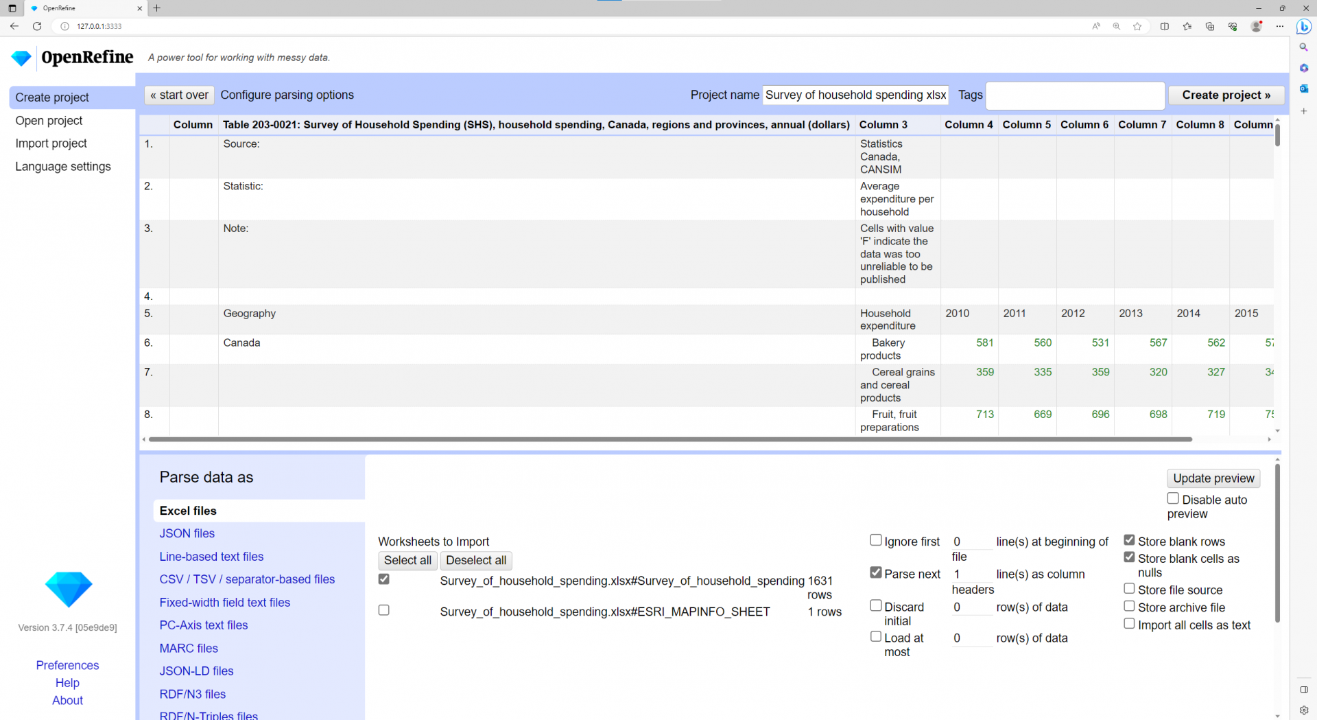
3. Ensure that Create Project is selected. Click on Choose Files. Browse to the file Survey_of_household_spending.xlsx. Click Open. Then, click the Next button.

4. You are now viewing the dataset in Preview view. Here you can see what data will look like when loaded, and make changes to what data OpenRefine will load.

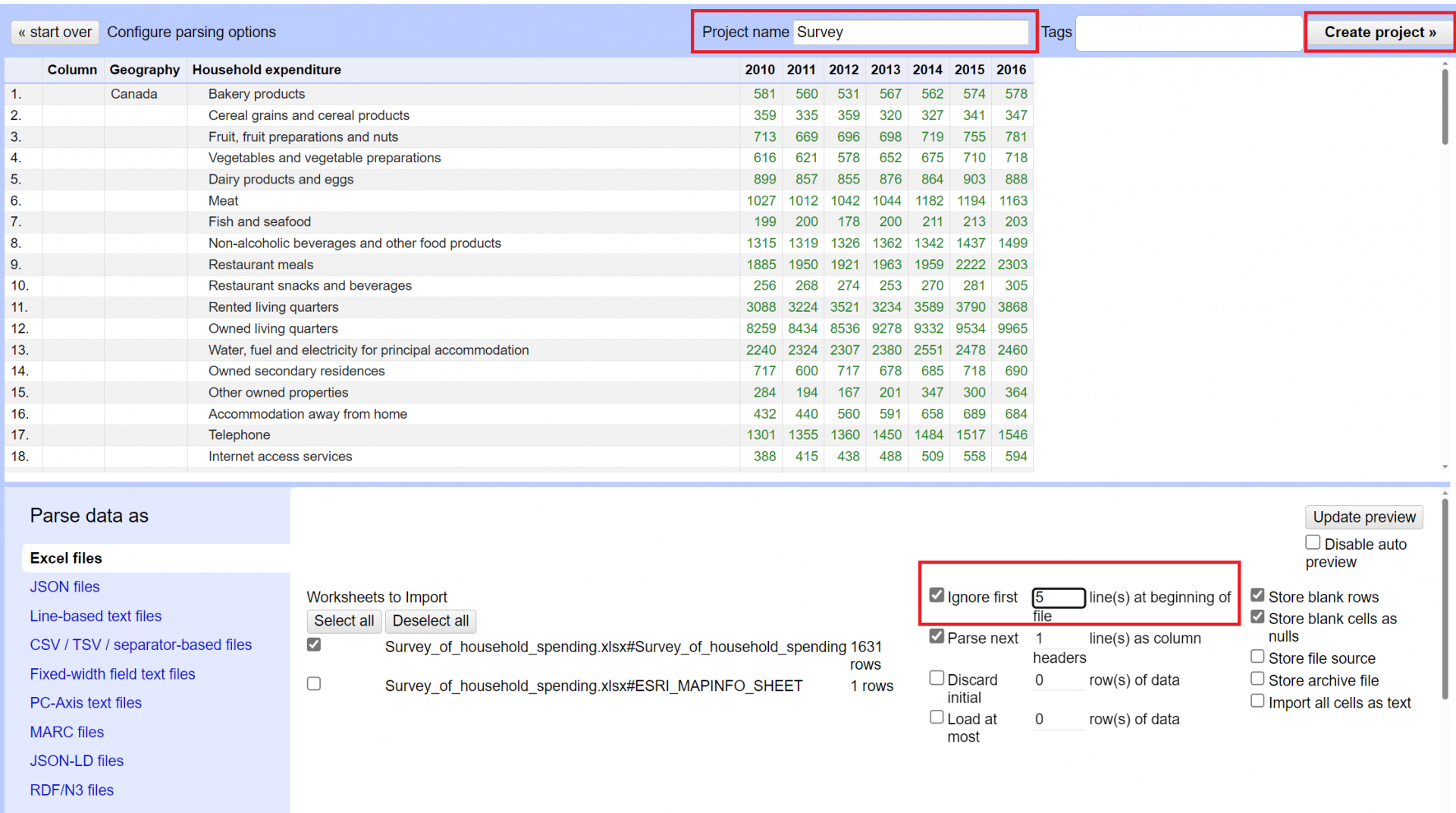
- Notice that the descriptive text at the top of the Excel worksheet is showing in the preview, and is messing up OpenRefine’s ability to identify the column headings. We can instruct OpenRefine to ignore these rows that aren’t part of the data table. Select the check box beside Ignore first, and type 5 in the box to ignore the first 5 line(s) at the beginning of the file. Click on Update Preview to see the changes.
- Notice also that numbers are displayed in green, this means OpenRefine has recognized these columns as containing numeric data (as opposed to text)
- In the Project name box, give the project a name of your choice.
- Click Create Project

5. Your data has now been loaded into OpenRefine.
Note: It has stored a copy of this data with the OpenRefine installation files on your computer. When you make edits using OpenRefine, you are not editing the original data file you uploaded, all edits are made to the copy OpenRefine has created.
Perform some basic data cleanup to get familiar with the OpenRefine interface
6. In the top toolbar, select 50 in order to show more rows on the screen at once.
7. Let’s remove the blank column. Look for the pull down menu (button with downward-pointing arrow on it) for the column named “Column”. From the pull down menu, select Edit Column > Remove this Column.

8. Now let’s take a look at the “Geography” column. We want to fill the entries down so that all rows have a geography associated with them. From the Geography column pull down menu, select Edit Cells > Fill Down. In the top toolbar, click Next a few times in order to look at a few pages of results. Verify that the fill operation seems to have worked.

9. Next, look at the “Household expenditure” column. Remember earlier we noticed that there were leading spaces? It appears that they are gone now. However, hover your cursor over a cell in this column and click edit. You’ll see that the leading spaces are still there. Click Cancel on the edit window. These “invisible” leading spaces could cause problems down the road, so let’s remove them altogether. From the Household expenditure column pull down menu, select Edit cells > Common transforms > Trim leading and trailing whitespace. Check a cell to verify that the leading spaces are gone.

Use OpenRefine to sort, filter and facet data
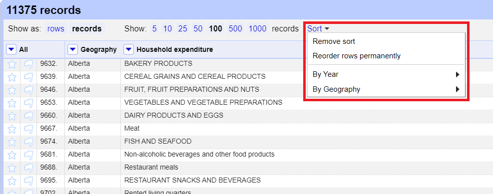
10. Rows of data are initially loaded in the order they appear in the original data file. In this case, they are grouped by geography, with Canada first, then going through the provinces from east to west. To change the sort, from the Geography column pull down menu, select Sort…

In the Sort window, sort as text, ordered from a-z. Click OK.

11. We could put a secondary sort on another column, such as 2016 expenditures. From the 2016 column pull down menu, select Sort…, and sort by numbers, from largest first. Notice the “sort by this column alone” option at the bottom of the window – that only appears when there is already one or more sorts in place. If you don’t check that option, it will keep the original sort and add this as a secondary sort. That’s what we want to do right now, so don’t check that box.

12. You can remove a sort at any time by pulling down the column’s menu, and choosing Sort > Remove sort. You don’t have to do this right now unless you wish to. You can also check what has been sorted and remove sorts from the top toolbar Sort menu that has appeared.


13. Filtering allows us to search for certain information within our dataset. Let’s say we want to display only the rows with a geography of Ontario. From the Geography column pull down menu, choose Text filter. The text filter appears in the left-hand sidebar, under the “Facet / Filter” tab. Type "ontario" in the search box. OpenRefine automatically removes any rows that don’t match from the display, leaving a total of 125 rows remaining (out of 1625 total).


14. We can have text filters on more than one column at a time. From the Household expenditure column pull down menu, choose Text filter. Type "clothing" in the search box for that filter. The two filters are combined, showing us all the clothing expenditure categories for Ontario.

15. You can remove a filter by clicking on the x in the top left-hand corner of the filter box. Remove both filters now. You should have all 1625 rows displayed again.
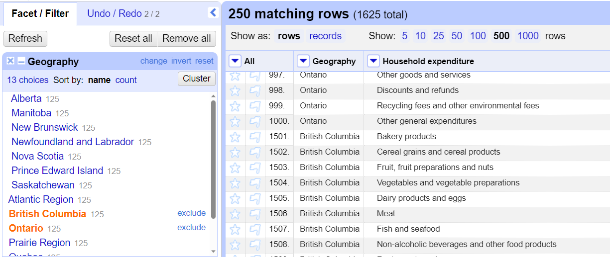
16. Next let’s explore an even more sophisticated way of selecting which data to work with. A facet summarizes all the values that appear in the column, and lets you select which data to view, as well as provides ways to edit the data. From the Geography column pull down menu, choose Facet > Text facet.

The facet appears in the left-hand sidebar, in the same area where the filters were previously. Have a look at the facet. It shows you how many total values there are in this column (13), how many rows contain each value (for this dataset it is the same for each, 125), and allows you to sort the values by name or by count (count won’t be helpful in this case since they all have the same count).

17. Click on Ontario in the value list. This has the same effect as using the text filter to search for Ontario, leaving 125 matching rows. However, from there we can do more than the filter allowed. We can select a second value at the same time. Hover your cursor over British Columbia in the value list and choose include. Now it is showing rows for either Ontario or British Columbia data. You can then exclude one or both of the selections at any time. Hover your cursor over Ontario in the value list and choose exclude. Now only British Columbia rows are shown.


18. Like with filters, you can combine multiple facets at the same time. Add another text facet on the household expenditure column. What did the average household in British Columbia spend on pet food in 2016? [You can find the answer at the end of this tutorial.] Once you have the answer, remove both facets by clicking on the Remove All button at the top left.

19. You’ve now seen faceting for text fields, but how can you work with numeric fields? From the 2016 column pull down menu, expand Facet, and look at the options. There are some other types of facets available, including numeric facets. If we created a numeric facet now, it would only work for this column, so you would have to facet each year of data separately. Let’s manipulate the data a bit first, and then come back and work with numeric facets.
Transpose the data from wide format to long format
20. What you have right now is “wide” format data. You should convert it to “long” in order to work with it using numeric facets. Converting to long format will put all the years into one column, and all the numeric data values into a second column. If that is confusing, let’s try it and you’ll be able to see what it does. From the 2016 column pull down menu, select Transpose > Transpose cells across columns into rows…

21. The Transpose window appears. You are going to put the data from the 7 numeric data columns (named 2010 through 2016) into two columns, one containing the year, and one containing the numeric data value (representing an average expenditure amount). For the From column choose 2010. For the To column choose 2016 (or last column, either will work). In the Transpose into section, we will use the Two new columns option. The Key Column will be the years – call it Year. Give the Value Column the name Average expenditure. Check the Fill down in other columns option. Click Transpose.

22. Have a look at the result. For each province, for each expenditure type, you now have 7 separate rows, one for each year. Notice your dataset now has 11,375 rows, compared to 1,625 before transposing. It has fewer columns, but many more rows – this is why it is referred to as a “long” format. Long format can be useful for certain types of data analyses, where all your data measuring the same thing (e.g., average expenditures) needs to be in one column instead of spread over many.

Explore more advanced uses of facets
23. Now that the data has been transposed, you can return to working with numeric facets. From the new Average expenditure column pull down menu, choose Facet > Numeric facet. Numeric facets provide a sliding scale where you can choose which values to include. Notice the blue areas indicate where the values fall – you can see where the bulk of your values lie, and where there are some outliers. Let’s try to remove the outliers by dragging the handles so the facet includes only the largest block of blue values. This removes a number of rows from the display.


24. Notice at the bottom of the numeric facet, there are options to show Non-numeric values, Blanks, or Errors in this column. There are no blanks or errors in this data column, but there are non-numeric values. Uncheck Numeric in order to look only at the Non-numeric values. Most of these have values of “F” in them, but some of them are actually blank! Why are they included here rather than counted as blank cells by the facet? Hover your cursor over a blank cell and click Edit. There are spaces in this cell – remove them using Edit cells > Common transforms > Trim leading and trailing whitespace. Notice in the facet that there are now a number of cells recognized as blank.

Note: in OpenRefine, any actions you perform are only applied to the rows currently selected, i.e., the above task was only applied to the non-numeric cells that are currently selected.
25. What does the “F” value mean? This was included in the information at the top of the original spreadsheet, which we removed when we loaded it into OpenRefine. If you were to go back and look at the Excel file you’ll see that “F” means the data was too unreliable to be published. If you wanted to change the value of “F” to be something more descriptive, you can use facets to edit data in bulk. However, we can’t do it from a numeric facet, we need a text facet instead. From the Average expenditure column pull down menu, select Facet > Text facet. Notice that only the non-numeric values are listed – this is because you still have only non-numeric values selected (via the numeric facet).

Hover your cursor over the value F and choose edit. Change F to something more descriptive, such as Unpublished. Click Apply. All values of F in the dataset are automatically changed to Unpublished.

Note: Another quick way to bulk edit data is to edit a particular cell, but then select Apply to All Identical Cells to make the same change throughout the column.

26. Then reset all the facets by click on Reset All button on the top left.
In summary:
Text filters are for free text searching, so that you can identify all rows that match your search string to a particular column value.
Facets are for structured viewing of the unique values in a column (including counts of unique values), filtering by those values (alone or in combination), and editing of unique values.
General Refine Expression Language (GREL)
27. I’d like to introduce you to one final major concept using this dataset – GREL or General Refine Expression Language. It’s a way of providing more complex instructions to OpenRefine than what you can do from the menu options. You can use it to do simple transformations on your data. In the Household expenditure column, pull down Edit cells > Transform...

28. One way you can use GREL is to do simple string manipulations, for example, type: value.toLowercase() – you can see in the preview that this command changes the value in the column to all lowercase letters.

29. Now try: value.toUppercase() – you can see the preview changes. Click OK.

So how to do you know what commands are available in GREL? If you just google GREL OpenRefine you’ll find a page that links to documentation on different GREL functions you can use. You can also just google GREL and what you’re trying to do to find help. This is just a basic intro – we’ll see some more examples a bit later.
Export Data from OpenRefine
30. In the top right-hand corner of the screen, pull down the Export menu and choose comma separated value (or Excel, or whatever format you would like to download).
Note: OpenRefine automatically saves projects, which you can access on the main OpenRefine menu by clicking on “Open Project” and then selecting the project you wish to continue. Exporting is for when you want to use your cleaned data in another program.

31. If you are on a Windows computer, you can close OpenRefine by first clicking on the black terminal window, and holding CTRL + C until it closes. The server that performs all of OpenRefine’s operations is now closed, and OpenRefine will not respond to further commands. You can now close the OpenRefine tab in your browser.
That’s it for our Statistics Canada dataset! You’re now familiar with the OpenRefine interface and basic functionality.
Answer for step 18 above: In 2016, the average household in British Columbia spent $361 on pet food.