Table of Contents

• Introduction
• Document Clustering
• Named Entity Recognition
• Ngrams
• Parts of Speech Tagger
• Sentiment Analysis
• Topic Modeling

Introduction

(back to table of contents)

1. Now that we have our text collection and our cleaning configuration, let’s try some tools. To get started, click on the Analyze button in the toolbar.
   

2. Under the Content Set dropdown menu, click on Select Content Set.
   

3. Select Stein.
   

4. Now, click Add Tool (at the top-right corner).
   

5. Here you can pick from Gale’s six tools. For this particular project, add all six tools: Document Clustering, Named Entity Recognition, Ngram, Parts of Speech, Sentiment Analysis, and Topic Modeling. This selection includes a mix of qualitative and quantitative tools.
   

6. Finally, click done.
   

7. The Analyze page now lists your chosen tools.

   Note: once you run the various tools, you can return to this page to view your analyses and visualizations.
   

Document Clustering

(back to table of contents)

1. On the Analyze page, under the Document Clustering tool, click Edit.
   

   Note: while there is an option to run multiple (or all) tools simultaneously, without prior setup, this option would use the default cleaning configuration. Since we made a custom cleaning configuration, and so that you can see some of the options for each tool, we’ll run each tool individually.

2. Just like with the cleaning configurations, you can customise your settings for each tool. Name the tool setup Stein Cluster, set the Cleaning Configuration to Stein, and set the number of clusters to 3.

3. Finally, click run.
   

4. The tool will then begin processing.

5. This analysis job is processed on Gale’s servers. Let’s wait a minute.

   Note: every tool has an About icon, which gives you a popup with some basic information and a link to fuller documentation. All of the tools in the Digital Scholar Lab are free tools you can download and run on your computer (sometimes they run on their own, other tools like Document Clustering rely on a programming language like Python).

   Click on the Help button for information about how this tool works.
   

   Note: the Document Clustering tool uses the Python programming language to run a Python library called SciKit-learn. It uses machine learning, specifically the k-means clustering algorithm, to group the documents based on their similarity in terms of vocabulary. 

   Go back to the Stein Cluster page. Then, Refresh the page (CTRL+R or F5 in Windows, Command+R on Macs.)

6. Once the Run Status says Completed, it should create a graph similar to this one:
   

   There are hundreds of dots on a scatter plot, in a roughly triangular arrangement, clustered into three colours: black, blue, and green. Each dot is an individual text, and the more similar two texts are (in terms of their vocabulary), the closer their corresponding dots are. Each cluster is colour-coded and uses a different symbol for each point.

   Note: Although there are scales on the X and Y axes, they have no meaningful numeric significance. Instead, they provide a reference for measuring distance or closeness between individual points. For more information on the mathematics of how this algorithm works, see this video on the k-means algorithm.

7. Mouse over one of the dots: a popup appears with the title of text you chose. Clicking will bring you to the Doc Explorer view of that text, but don't do that, as we want to look at the corpus as a whole.
   

   If you do click on any one of the dots, the Doc Explorer view will show you the document as well as 20 more documents that are most similar to it.
   

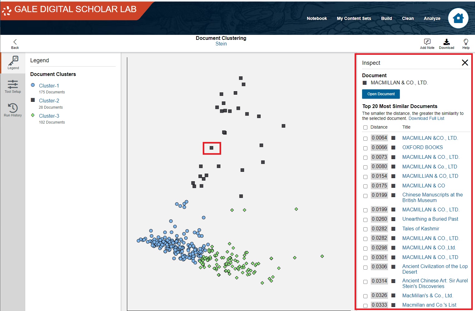
   You can check or uncheck any of the listed documents to add them to your content set. To do that, have the desired documents selected, scroll down to the bottom of the list, and click on 'Add to Content Set'. However, at this point of the tutorial, let's exit the Doc Viewer by clicking on the 'x' at the top of the list.
   

8. Now, a word of caution: what looks similar to the algorithm might not be meaningful to humans. In our case, however, there are some meaningful differences that look to me a little bit like different genres. Mouse over several of the dots and see if a pattern emerges. It looks roughly like Cluster 1 consists of short notices and bulletins, including biographical details (Stein’s publications and obituary). Cluster 2 contains brief reports of his expeditions and discoveries. Cluster 3 seems to be reviews of his published books. Note also that a number of book advertisements with similar names (MacMillan and Co) are clustered together, showing that the clustering tool recognises that they are similar in terms of their vocabulary.

9. For this scatter plot, you can download both the graph itself and the data used to generate it. On the toolbar, click Download. 
   

10. On the Download Options window that appears, under Visualization download formats, select PNG and then click Download.

Named Entity Recognition

(back to table of contents)

1. Let’s try our second tool. Click on Analyze. 

2. Then under Named Entity Recognition, click Edit.
   

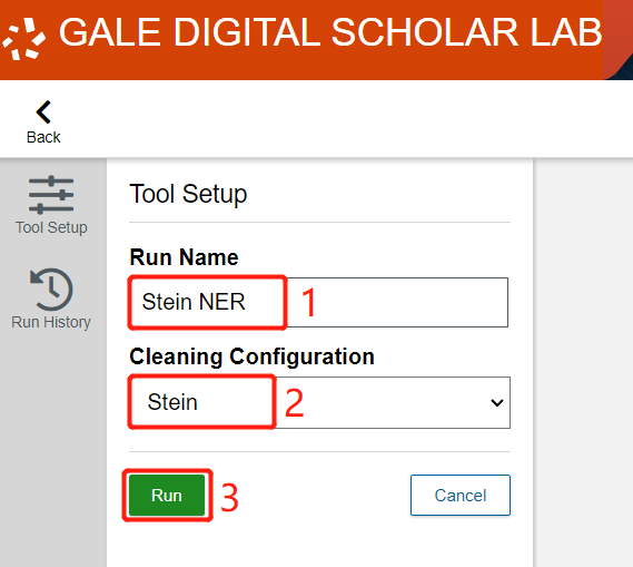
3. The Named Entity Recognition tool will extract common and proper nouns from our texts, and then attempt to classify them as people, titles, places, political entities, and so on. Name our tool Stein NER, set the Cleaning Configuration to Stein, and click Run.
   

4. While you wait, feel free to click on the Help button for information about how this tool works.

   Note: Named Entity Recognition uses a tool called spaCy, which runs in the Python programming language. It breaks up sentences into their component words, and then classifies the nouns. By default, it uses an existing vocabulary, and then tries to predict from context what classes new nouns fall into. It then tags and colour-codes these categories, and tells us where these terms can be found in our corpus .Click refresh and then you will see the results.

5. The Named Entity Recognition tool displays the set of nouns with the highest count across your corpus. The algorithm has classified, or in some cases guessed, into which category each word falls. Looking over the first few entries, it looks fairly good: it has correctly identified that "Chinese", "British", "Indian", and "Soviet" refer to cultural groups, that Aurel Stein is a person, and that "today" is a date. There are some issues, likely due to the unfamiliar terms: “Kashgar” is actually a city, not a person, but most entries are correct. I doubt that Kashgar, a Central Asian city, appears in the tool's default dictionaries, so in this case the tool guessed that Kashgar was a person based on its usage in various sentences.
   

   You can click on any entity for more information about where it appears in our corpus, and what other categories it also falls into. Let's try this.

6. Click on the first entry, Chinese.
   

7. Let's examine the results for this particular named entity.
   

   At the top, "Chinese" is identified primarily as a Cultural Group, which means that in your corpus, "Chinese" most frequently refers to groups of Chinese people or officials. Because Stein was primarily travelling through western China, often dealing with Chinese officials and manuscripts in Chinese, it makes sense for it to be the most common entity and also for these three meanings to dominate.

   In the second section of the popup window, there is a list of all documents in the corpus in which the term "Chinese" appears.

8. Click on "A Chinese Expedition Across the Pamirs and Hindukush A.D. 747." 
   

9. Click on the Open Document Button. Gale DSL will then present you with a view of the document, marked up with tags showing how it has identified each entity within the document.
   

   

   Note that this version of the text has been filtered through the cleaning configuration, so punctuation and common words (e.g. "the") are missing.

   Now that you have seen how Named Entity Recognition works on a particular document, close this window by clicking on the X.

10. You will now return to the popup for the term Chinese. Another feature available in the Digital Scholar Lab is to use the Named Entity Recognition tool to identify documents related to a single topic, and then create a new collection with some or all of the documents with that term. Let's say that you are interested specifically in Stein's relationships with the Chinese and want to create a sub-collection focusing on Chinese art and archaeology. Check the boxes next to "A Chinese Expedition Across the Pamirs and Hindukush A.D. 747," "Exploration in Central Asia," "Buddhist Paintings at the Festival of Empire," and "The Treasures of Asia." Then scroll to the bottom of the list to click on 'Add Selected'.
    
    

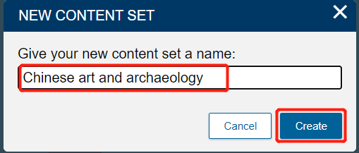
11. You can either add these documents to an existing content set or create a new one. Select "New Content Set";
    

12. name it "Chinese art and archaeology".

13. Now, close the notification by clicking the Close button.

    Note: you can check to see the new collection by clicking on My Content Sets. Named Entity Recognition provides an additional way of creating content sets outside of searches. Be sure to return to the Named Entity Recognition tool to continue with the next step.

14. There are many categories that aren’t helpful right now, so let’s filter so that we just have categories we’re interested in. First, uncheck Category.
    

15. Then, check Geo-Political Entity, Person, and Cultural Group.

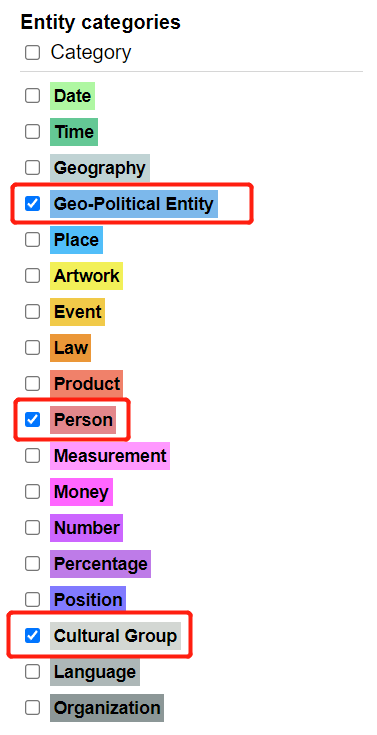
16. You will now have a list consisting of just those three categories.

17. Now we can begin to answer questions like, “Which cultural groups are mentioned most often in association with Aurel Stein?” or “Who associated with him? Who does he write about?” As with the Clustering tool, you can download the complete data for further analysis by clicking on the Download button.
    

18. Although there are no data visualizations, like graphs, you can download the data as either CSV (a spreadsheet) or JSON. Click on CSV and then Download.

    Note: this dataset might need some cleaning, as you saw with the city of Kashgar being incorrectly interpreted as a person.

Ngrams

(back to table of contents)

1. One popular tool is Ngrams (you might know of it through Google Ngram Viewer), which counts the frequency of specific words in a corpus. Click on Analyze and then click Edit under the Ngrams tool.

2. You’ll see that the Ngrams tool has a few settings. Let’s change the Name to Stein Ngram and the cleaning configuration to Stein; leave the Ngram sizes at their defaults (min 1, max 6); set Ngrams Occurence Threshold to 5; and return 75 ngrams. Finally, click run.

3. The Ngram tool counts the number of times a term or a phrase occurs in our corpus and then graphs it. The Ngram size option refers to the length of the term: 1 means a single word, whereas 3 means that it looks for three-word phrases. By default, the tool looks for single words or phrases up to four words long. Ngrams Occurrence Threshold is the minimum number of times a word or phrase must occur in the corpus to be part of the Ngram. By setting it to 5, we cut out words or phrases that occur just two or three times in our thousands of documents. Number of Ngrams Returned determines the number of terms that appear in our visualizations. The default is 1000 but we've reduced that to 75 for visualization purposes. Although you might want to know the top 1000 terms for your research, it can look a bit cluttered in a wordcloud. One key point is that this tool ignores any terms that are composed entirely of words from our stop word list. Once a minute has passed, refresh the page.

4. Now the word cloud and bar chart are both available. Click on the word cloud.
   

5. This image visualizes the most common words in the corpus, while accounting for our specific cleaning configurations and tool settings.
   

   If you mouse over a term, you can see how many times it appeared.

   Interpretation: the more frequently an ngram appears in the corpus, the larger it appears in this word cloud. As we saw with the Named Entity Recognition tool, Chinese (referring to Chinese culture, Chinese people, and the Chinese language) are major topics in writing by or about Stein. In addition, British, Majestys (i.e. "In His Majesty's Service"), Subject(s), and other terms referring to British imperialism from 1900-1940 appear. There are several terms related to specific places (e.g. Kashgar) and official positions (e.g. Taoyin, Amban) in China or the Chinese government. Since Stein recorded his travels, many words related to geography (route, river, stream, valley, pass, road, ground, bank, etc.) occur. "Russian" and "Soviet" are also major terms because the British Empire was competing at this time with Russia (both imperial and then later Soviet) for control over the territories between British India and Russian Central Asia. (For more information, see The Great Game.)

6. Word clouds are popular and it’s useful to be able to generate them. Click on Download.
   

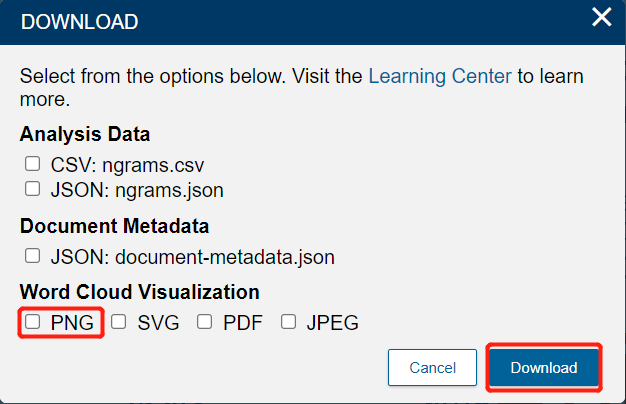
7. Here you can download either the Word Cloud image or the underlying data from the Ngram tool (which lists the most frequent words and phrases in the corpus). Let's download the image as a PNG. Click on Term Frequency PNG and then Download.

   Note: unfortunately, there is no way to control the position or colour of specific words - they appear to be randomly generated. By resizing your browser window, you resize (and thus randomly reposition) some of the words in the world cloud.

8. Let’s switch to the bar chart. On the top menu, click on Bar Chart. Note that the "Rank" view sometimes create better visualizations.
    

9. This provides another way of looking at word frequency. Here, we can see at a glance which words were most popular. 
   

   "Chinese" is the most popular word by far, which makes sense considering that Stein was travelling extensively through China and interacting with Chinese officials. Kashgar, a city in western China where both the British and Russian consulates were located, is the second-most common term. Stein actually comes fourth, which is surprising considering these texts are specifically about or by him. "Road" and "river" come fifth and sixth, likely because Stein was writing about the geography of these locales. Ngrams are one of the simpler text analysis tools but they can reveal a great deal about our text collection.

Parts of Speech Tagger

(back to table of contents)

1. The Parts of Speech Tagger compares the writing styles of different authors by counting their use of different parts of sentences, such as proper nouns and adjectives. Begin by clicking on Analyze in the top menu. If necessary, select Stein from the dropdown menu. 

2. Under the Parts of Speech Tagger tool, click Edit.

3. The cleaning configuration we have created removes many parts of speech that this tool counts. In order to show how cleaning configurations affect this tool, and to better understand the various authors' styles, we'll run this tool twice, once without a cleaning configuration, and once with. Begin by naming this tool setup "Stein no cleaning". Change the cleaning configuration to None. Then finally, click Run.

4. Wait for a minute, then refresh. With the tool complete, DSL will produce a graph comparing the content sets. Each tick on the X-axis represents a different part of speech - pronouns, proper nouns, adjectives, etc. - and the Y-axis represents their frequency.
    ​​​​​​

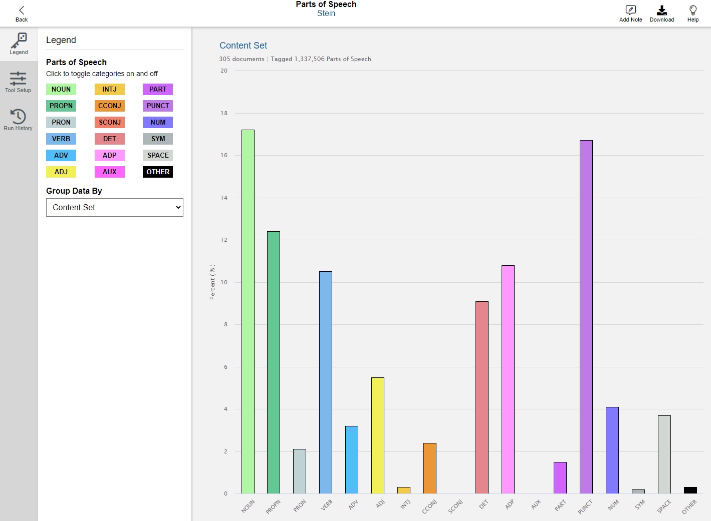
5. This is a useful start, but it is too cluttered. We want to look into the styles of different authors. On the left sidebar, click on the dropdown menu and select Author.

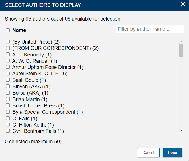
6. To show the styles of authors that we are interested in, click on Change selection to change the filter for authors.
   

7. First, uncheck all the boxes (the first ten boxes)

8. Now the filter would look like this:​​​​​​​

9. In the top-right Author Filter box, type "stein" (without quotation marks). Select "Sir Aurel Stein.", which should be the third option. Leave off the others.
   

   Note: Stein's name appears several times here because his name has been entered with variations in the documents in DSL. This tool treats each variation of his name as a different author. The variation we chose above is associated with the most texts.

10. After adding Sir Aurel Stein, type "Giles" in the Author Filter. Add "Dr Lionel Giles". The author will be added to the accompanying graph.
    

    Note: Lionel Giles was a contemporary of Stein's, and was a scholar who worked at the British Library. His name appears twice because in one text, "Lionel Giles" and "Lionel Giles;" The one without semicolon) is added as author. 

11. Type "Mirsky" in the Author Filter and add Jeannette Mirsky.
    

    Note: Jeanneatte Mirsky wrote a biography of Stein in 1977. Although she's writing about similar content as him, she wrote much closer to the present day, so any differences revealed by the Parts of Speech Tagger are likely due to their different styles rather than content.

12. Type "Lattimore" in the Author Filter, and add Owen Lattimore.

    Note: Owen Lattimore was a scholar of Asia, but his writing style differs markedly from Stein's.

13. Finally, click Done to see the complete legend. Four bar charts that describe the writing style for each author are shown. The final version of this graph reveals some major differences in writing styles: for example, Lattimore uses a much higher proportion of proper nouns than anyone else.​​​​​​​
    

14. Now, let's try rebuilding this chart, but with our existing cleaning configuration. In the left sidebar, click on Tool Setup. 
    

15. Below the existing tool setup, click on New tool setup.​​​​​​​

16. Name this setup "Stein with stopwords". Change the cleaning configuration to Stein. Finally, click Run.
    

17. Wait a minute, then refresh the page. Just as before, use the Author Filter to add Aurel Stein, Lionel Giles, Jeannette Mirsky, and Owen Lattimore. Deselect all other authors. Now there are practically no conjunctions, particles, adpositions, or pronouns. As a result, some of the other parts of speech take on proportionally more weight. It is up to you as a researcher to determine which cleaning configuration - or none at all - works best for your aims. 
    

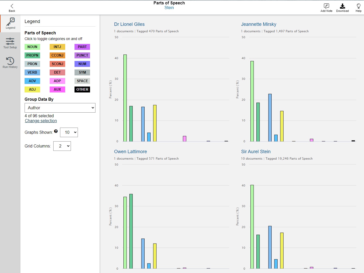
    Note: When in doubt, using no cleaning configuration is best for the Parts of Speech Tagger tool.

That's it! You have learned how to use the Parts of Speech Tagger to begin comparing the styles of different authors, and you have learned what kind of impact the cleaning configuration has on your data.

Sentiment Analysis

(back to table of contents)

1. Sentiment Analysis is a powerful tool for estimating the overall positive or negative emotional feelings of thousands of texts very quickly.
   On the Analyze page, under Sentiment Analysis, click the edit button to edit tool setup
   

2. In the Tool Setup for Sentiment Analysis, call the tool setting "Stein Sentiment", change the cleaning configuration to Stein, and finally, click Run.
   

3. As always, you can click on the About button to get more information.

   Note: Sentiment Analysis works by analyzing the words in a sentence, and looking them up in a dictionary that has a positive or negative score for many words. For example, the word "good" has a score of (positive) 3, and the word "unhappy" has a score of -2. The tool sums all scored words in a document and DSL then groups documents by year and averages their scores to produce yearly scores. You can download the full word list and their associated scores from AFINN. Note that Gale upgraded the version of the AFINN lexicon on July 13, 2023 to AFINN version 165. Rerunning earlier analyses with the new version of the tool may provide different results.

   Warning: the sentiment analysis tool does not understand context or meaning. It cannot distinguish sarcastic statements from sincere ones and it will not recognize words not on its list. Furthermore, without additional coding, it does not recognize negations, e.g. that "not impressed" means roughly the same thing as "unimpressed." It also embeds certain cultural assumptions and values: one of the example phrases in the Python code used to run this tool is "Rainy day but still in a good mood," where "good" is +3 and "rainy" is -1, for a sum of 2 for this sentence. The speaker might actually enjoy the rain, but this tool cannot account for that. These criticisms do not mean that the tool is useless, but that it is most effective when dealing with a large number of relatively straightforward texts. Like all tools in the DSL, it can be powerful (giving a rough estimate of the sentiment of thousands of texts within a minute is beyond human ability) but you need to understand how it works (and where and when it does not work).

4. Refresh the page. It may take minutes to process. Let's take a look at the results:​​​​​​​
   

   The x-axis represents years, and the y-axis represents the average sentiment score of all texts for a given year. This means that each point is an average of all words in all of the texts for a given year.

5. You can get more information about specific years by clicking on the associated point. Find the point for 1920 and click on it.
   

6. A popup will list all documents associated with a specific year. Some years have many associated documents, whereas others have only one. You can click on document titles to go to the page for that document. Once you are done, click X.
   

7. Some years have extreme scores, either very high or very low. Click on the point for 2011, which is the rightmost point.
   

8. There is only a single document for 2011. In general, since DSL averages the scores of all texts for each year, the most extreme points (the highest and the lowest) often have only one text. Let's investigate further. Click on the document title, "Turkey." DSL will open the doc explorer view. This text actually has almost nothing to do with Stein - it mentions him once in passing - and instead is a rather negative review of an unrelated book. Return to the Sentiment Analysis tool and click Close.
   

9. We can have more useful results by removing documents like these. Let's create a new collection that is a subset of this one. On the top toolbar, click My Content Sets.
   

10. Click on New Content Set.
    

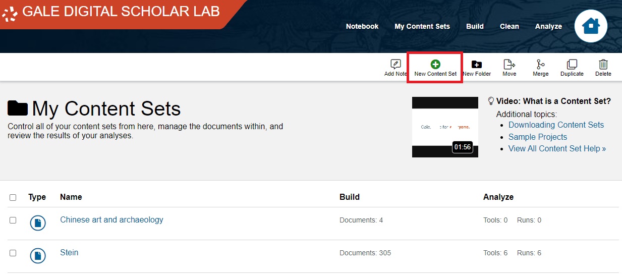
11. Name it Stein sentiment.

12. You should now see it in your list of content sets. Do not click it yet, though.​​​​​​​​​​​​​​

13. On the top toolbar, click Build. Then, on the Build screen, near Search, click View all limiters in Advanced Search.

14. Keep all three rows set to the Keyword field. Change the operators to OR. For each of the three fields, type Aurel Stein (as with the first content set) and pick one of the three versions of his name for each row.
    

    ​​​​​​​​​​​​​

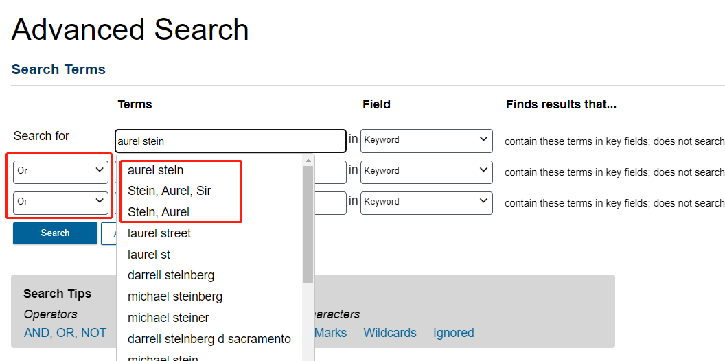
    However, once you are done, do not  click search. We are going to add more qualifications to remove problematic documents.

15. Scroll down. Under More Options, and under Publication Year, pick Between. For the first dropdown menu, type "1890" and press Enter. For the second year, type "1950" and press Enter.
    

16. Under publication language, pick English. Then, click Search.

17. On the search results screen, underneath All Content, check Select All.
    

18. It will then say that "All 100 results on this page are selected.

19. Click on "Select All (239) results." Remember, your document count may be different. 
    

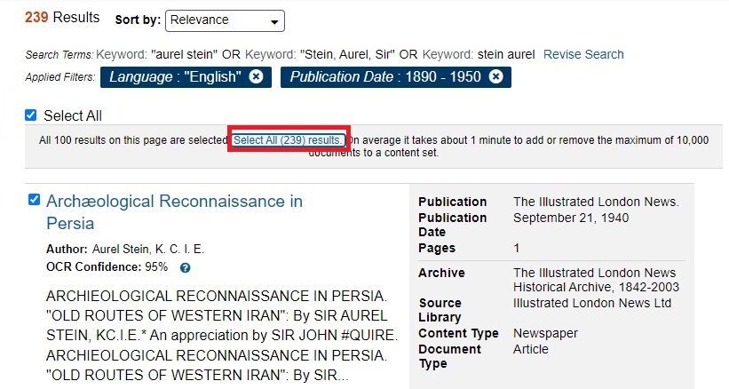
20. Now it should say, "235 results are selected." Make sure that the Active Content Set is set to "Stein sentiment".
    

21. Then, click the "Add to content set" button in the top and click Stein sentiment Content set.
    

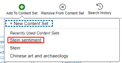
22. There should be a popup that says "Added 239 document(s) to Stein sentiment." Click View Content Set.
    

23. Since advertisements often include very positive language for marketing reasons, and since several of the advertisements in this collection only mention Stein briefly, we will improve our sentiment analysis by removing them. 

    Once you are in the Stein sentiment content set, click Documents.
    

24. On the right menu, under Document Type, click on Advertisement.​​​​​​​
    

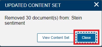
25. Once you are on a screen with only the advertisements, under Documents, check Select all on page. Then, on the top right of the page, click on Remove from Content Set.
    

26. There will be a popup that notifies you that these documents have been removed from Stein sentiment. Click Close.
    

27. You've trimmed your content set down to something more focused. On the top toolbar, click on Analyze.
    

28. Change the content set to Stein sentiment if you are not there already. Then, click Add Tool.
    

    Note: Remember that since this is a new content set, you have to add tools again, but we'll only add Sentiment Analysis for this content set. We'll return to the previous content set for the next tool.​​​​​​​

29. And add just the Sentiment Analysis tool, then click Done.
    

30. Under Sentiment Analysis, click Edit.​​​​​​​​​​​​​​
    

31. First, name this tool setup "Stein sentiment 1890-1950 no ads". Second, set the cleaning configuration to Stein. Third, click Run.
    

    Wait, refresh, and the result will be shown in a minute.

32. On average, there are more now documents per year. After removing ads and texts from considerably after Stein's life, the remaining texts are more representative. Explore by clicking on the various points.
    

33. One year in particular stands out for having a large number of texts with a largely negative sentiment. Click on the point for the year 1931.
    

34. Stein had three well-regarded expeditions to western China and Central Asia. In 1931, though, his fourth expedition was halted soon after it began when he was expelled from China. Here you can see a large number of newspaper articles reporting on this event. Click on X once you are done.
    

    ​​​​​​

    That's it for Sentiment Analysis! You learned how to use it, interpret the results, and how to use an advanced search to create a subset of your collection to improve the tool's results.

Topic Modeling

(back to table of contents)

1. The final tool in the Digital Scholar Lab is Topic Modeling. Before we use this tool, we need to modify our Cleaning Configuration, because Topic Modeling is case sensitive. This means that it will consider capitalized words to be different from uncapitalized ones. At the top toolbar, click on Clean.​​​​​​​
   

2. Click on Stein under Your Configurations.​​​​​​​
   

   Note: my screen displays many more Cleaning Configurations than yours will. This is for testing purposes, but you only need to have the Stein configuration.

3. Under Text Modification, check the box for All lower case. Then, click on Save As on the upper toolbar.​​​​​​​
   

4. Name the new cleaning configuration "Stein lower case", then click Submit.
   

5. Now, let's use this new cleaning configuration in the Topic Modeling tool. Click on Analyze (top toolbar) to get back to the analysis menu, and change the Content Set back to Stein (if it isn't already).​​​​​​​
   

6. Then, under Topic Modeling, next to Run Details, click Edit.
   

7. Name this tool "Stein Topics", set the Cleaning Configuration to "Stein lower case," and increase the Number of Topics to 20. Leave Words per Topic and Iterations at their defaults. Click run.​​​​​​​
   

8. Once a couple minutes have passed, refresh the page.

   Note: The Topic Modeling tool uses a free program called MALLET, which stands for Machine Learning for Language Toolkit. MALLET uses an algorithm called Latent Dirichlet Allocation, or LDA for short. Basically, it looks for words that occur together often in the corpus, and then brings them together as a “topic.” This tool uses a certain degree of randomness, which is offset by running the tool many times in the background - this is what the Number of Iterations refers to. If you would like to install MALLET on your own computer, use this MALLET installation guide and tutorial.

9. If your tool defaults to the "Topic Proportion" screen, click on the "Topics" icon in the top left. We'll come back to topic proportions after working more closely with our individual topics first.​​​​​​​
   

10. On the "Topics" page, you will have twenty topics, numbered from 0 to 19. Each lists the words that appear together most frequently. The topics will also display as a horizontal bar chart, with one of several Topic Metrics displayed. The default is Average Word Length.​​​​​​
    

11. Click on the Topic Metric dropdown menu, then on each of the metrics in turn, considering how the other options affect your results. Each of these metrics may help identify topics to avoid or focus on.
    ​​​​​​​

    Average Word Length measures word length, with longer words suggesting more specific (and therefore meaningful) topics.
    Coherence measures the likelihood that words within a topic appear next to each other.
    Corpus Distance measures the distance from words in a topic from the corpus as a whole, suggesting which topics are most distinct from the rest of the corpus.
    Document Count displays how many documents appear in each topic. Topics with just one or two documents might be outliers, but topics that appear in the entire collection might be too vague.
    Document Entropy measures the probability that each topic appears in a randomly selected text.
    Exclusivity measures how often the top words in a topic co-occur with top words in other topics.
    Tokens measures how often words from specific topics appear in the entire corpus.
    Uniform Distance suggests which topics are the most specific.
    When you're done, select Average Word Length again.

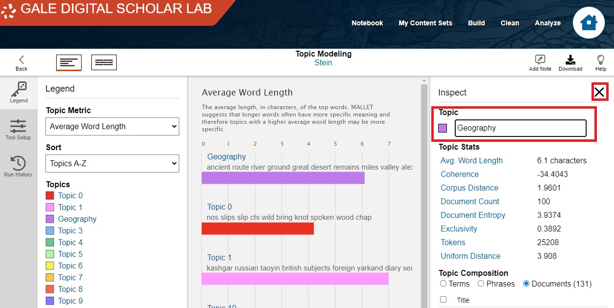
12. If you scroll through the list of topics, most topics should look like they refer to similar topics or themes. There’s a bit of randomization in this tool, so your topics and their numbering will vary from those in these examples, but the large number of iterations ensures that most of the time, the tool produces topics that are fairly similar to each other. Here, my topic 2's words are river, road, route, pass, valley, small, stage, bank, stream, and path. They appear to have a strong focus on geography and travel. Pick any topic and click on it. 
    

    Note: for the purposes of this example, I will demonstrate using my Topic 2, but you can pick any topic.

13. This will display the Inspect pane, where you can rename the topic, consult its summary statistics (Average Word Length, Coherence, etc.), consult statistics for each of the top terms (e.g. how common is "river"? how many documents does it appear in, in the context of being part of this topic?), and switch to displaying Phrases and Documents. Click on Documents.
    

    You will then have a list of all documents in which this topic appears, which is helpful for determining the genres and content of this topic. As you might have suspected, my topic 2 has a number of documents related to both Stein's travels and those of others (e.g. Alexander the Great), along with texts like "Ancient Ways in Iran" and "Routes in Sinkiang" (i.e. modern Xinjiang Province in western China). If any of these documents interest you, you can click on them to view them, making the topic modeling tool another method for discovering primary sources.

14. Now that we have confirmed this topic's strong focus on geographic texts, let's name it Geography. Click on the topic's title and rename it "Geography", then click X to close the pane.
    

15. Go through the list and give titles to each of the topics. You should be able to guess at the general theme of most topics, especially if you consider which documents appear in each topic.

    Another example is my topic 12, which includes words like "Soviet," "bureau," "agent," and "intelligence." These suggest the British government's involvement in the Great Game, particularly intelligence gathering, so I named this topic "Intelligence Gathering." I drew on my own domain expertise to identify this; when using topic modeling for your own research, you will likely also make connections that someone unfamiliar with your topic might not notice.

    Note: it is very likely that one or two of your topics resembles my topic 6, with non-English words like "gyappa" and "nangwa" included alongside the word Tibetan. If you click on "Identified in: 2 Documents," you will likely see two English-language textbooks for learning Tibetan. These topics thus include a number of Tibetan words, grammatical terms, and words like "tea" that are occur frequently in the example sentences in these books. Feel free to name this topic Tibetan.

    If there are any topics which are unclear, feel free to leave them untitled, label them "unclear" or "junk", or to add a question mark at the end of the topic name - anything that lets you, the researcher, know that the topic is ambiguous. Sometimes topic modeling groups words together that have no meaningful connection; other times, a topic might seem vague, but further research reveals a connection.

    Note: clicking on the Download button here allows you to download the data for each of these topics. If you are in the Topic Proportion view described below, you will have access to different download options.

16. Now that we’ve seen roughly what words and themes our topics cover, let’s look at how common these themes are in our corpus. In the top left corner, click on the Topic Proportion icon.
    

17. The Topic Proportion page displays a horizontal proportional bar chart. Each row represents a single text in our collection, with a total for whole Content Set at the top; each bar is colour-coded to show which topics appear in that text and in what proportion.​​​​​​​
    

18. By default, the Digital Scholar Lab displays the first fifteen documents in your collection. Let's change that: scroll down and click on Selected Documents.
    

19. Uncheck all of the documents, scroll down, and check "Link with Kipling," "Kashgar: Monthly Diaries (1912-1920)," "In Track of Alexander the Great," "News in Brief," and "'New' China and Sir Aurel Stein." Then click Done.
    

    The Topic Proportion page now displays only the documents we've selected. Note that they are represented as being composed of different topics.

20. You can hover the mouse cursor over specific coloured segments to see which topic they correspond to, and what percent of that particular document is composed of that topic. You can click on a specific topic to display just that topic, making it easy to compare one topic's prevalance across your selected documents.

    Hover over a few topics to view their name and percentage.​​​​​​​
    

21. Then click on a topic of your choice.​​​​​​​​​​
    

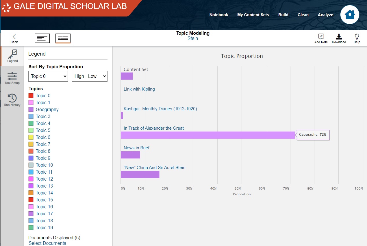
    This option displays only the proportion of this topic across all selected texts.
    Remember that on the Topic Proportion page, the Download option gives you different results than on the main Topics page. This is useful if you want to show the proportion of a specific topic in your collection.

That's it! You've run topic modeling, begun familiarising yourself with the metrics available, named your topics, explored the documents within them, and visualised the proportions of topics within various texts. You can use topic modeling to discover themes connecting texts and to identify specific documents that you may wish to read closely.

Continue to Exporting your results
Return to the main Gale Digital Scholar Lab tutorial