Once you have a dataset ready to analyze[1], the first step of any good empirical project should be to create summary statistics. This workshop is designed to teach you syntax, rather than point and click commands. The main advantage of writing a do-file is that you can always reuse most of it on different projects, with only a few tweaks; if you use Stata by point and click commands, you will be condemned to start from scratch every time.
We will use a dataset from the Canadian community health survey (CCHS). You can find it in the folder [insert path here, the dataset is U:\STAFF\JL\Stata\summarystatsproject\summstats.dta, a subset from CCHS I created and cleaned a bit (recode to make binary 0-1)]. Before we get started, let’s look at the description of each variable[2]:

Tabulate
A simple tabulation should always be your first stab at your data. The tabulate command returns a frequency and cumulative distribution table in the Stata viewer. Let’s say you want to know the proportion of respondent in the sample that ever got a flu shot:
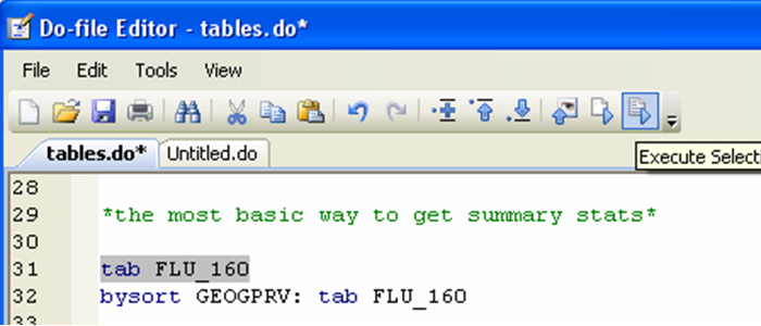

Note that you can combine the tabulate command with the by (or bysort) prefix to look at the tabulation for subgroups in your dataset. The prefix “bysort” is a combination of “by” and “sort”; you could equivalently break it into two commands, but it is generally simpler to use "bysort" Stata will first sort the data, then return the information by category. For example, here let’s see if the patterns of flu shots look different for each province:
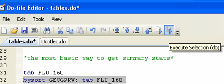

If you are interested in only one subgroup, you can also use the “if” qualifier with the tabulate command. Here, let’s say we want to know the frequency of flu shots in the sample for Ontario:
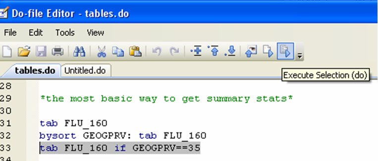

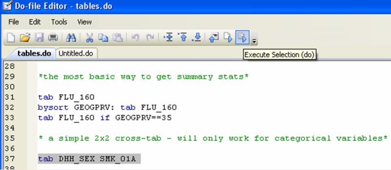
Finally, you can use the tabulate command to do a simple cross-tabulation using categorical variables. Say you want to know how many of the women in the sample smoked over 100 cigarettes in their life:

Summarize
Once you have tabulated your data, you can start looking at summary statistics other than frequency. The summarize command returns mean, standard deviation, minimum, maximum and frequency.
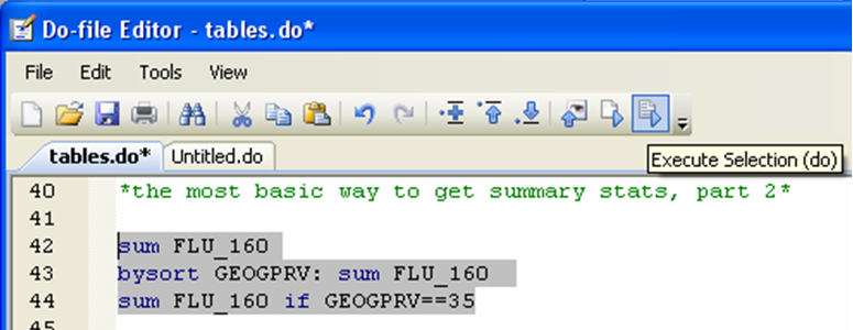
The example is built the same way the tabulate example was. First we look at the summary statistics for the whole sample, and then we look at the statistics for subsamples (each province).

Using the “if” qualifier returns the summary statistics for a specific subgroup.

In these examples we have focused on splitting the sample by province, but any categorical variable can be used. In subsequent examples, we will look at men and women, smokers and non-smokers, physically active or not. The way you look at your data depends on the type of questions you want to ask; the clearer your question, the more specific your analysis can be.
Tabulate, Summarize()
This combination of commands let’s you create simple one-way and two-way summary statistics tables in Stata.
The first part of the command (tabulate) will split your data according to a categorical variable (here we will use sex). The second part will give summary statistics for another variable (preferably quantitative). Let’s say you want to know how (whether) men and women differ in their daily consumption of fruit and vegetables:
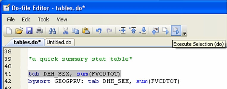
This table will give us the mean, standard deviation and frequency of the daily consumption of fruit and vegetables for men and women in the sample:

If you want to know whether men and women from different provinces have different patterns in their average daily consumption of fruit and vegetables, you can use the bysort command again to do the same query province by province:
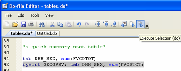

Note that you can also use the “if” qualifier here (as we did in the tabulate and summarize commands) to look at, say, one province only[3].
You can also use the tabulate, summarize() command to create a quick four-way summary statistics table. For example, if you wanted to look at patterns of daily fruit and vegetable consumption for men and women with different smoking habits, you could create a table for that:

The result seems to show a certain pattern: smokers look like they eat less fruit and vegetables than non-smokers, and women seem to eat more fruit and vegetable than men, on average[3].

Tabstat
The tabstat command displays summary statistics for a series of numeric variables in one table, possibly broken down on (conditioned by) another variable. Without the by() option, tabstat is a useful alternative to summarize because it allows you to specify the list of statistics to be displayed. With the by() option, tabstat resembles tabulate used with its summarize() option in that both report statistics of varlist for the different values of varname. The tabstat command allows more flexibility in terms of the statistics presented and the format of the table.

The first line will return the statistics (mean, standard deviation and frequency) for 4 variables (HWTGHTM HWTGWTK HWTGBMI PACFD) for the whole sample. The result window looks like this:

The second line tells Stata to do the same, but to split the sample between male and female. This is the result:
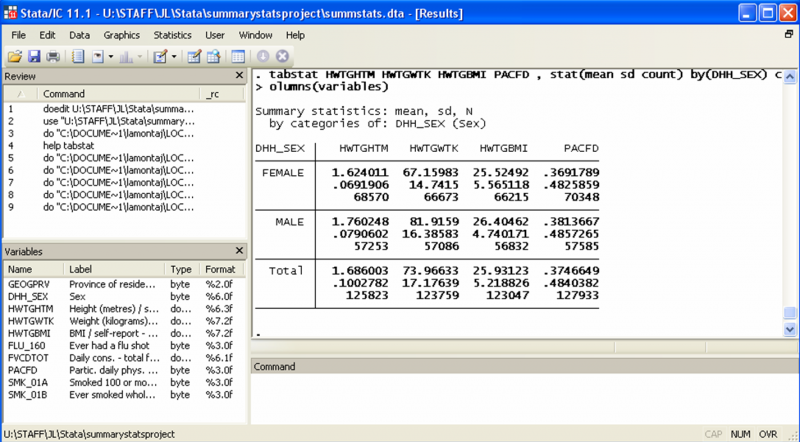
Notice how we also get the total, so if you are interested in the split samples and the total, no need to do both separately.
Finally, the third line of command, with the bysort prefix, will do the same in turn for each province, and split each sub-sample into male and female. The results are in the same format, however this returns subsample (i.e. provincial) total for male and female combined, but not the grand total for all provinces:

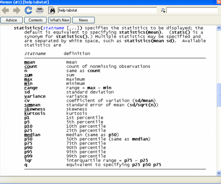
Note that you pick the statistics that are reported in the table. The statistics available are listed in the help tabstat:
Table
The table command calculates and displays tables of statistics. Just as in tabstat, you can pick the statistics you want reported, but you also choose which variable you want statistics reported for, as well as which variables you want the information cross-tabulated by. The structure of the syntax is simple but bears a closer look:

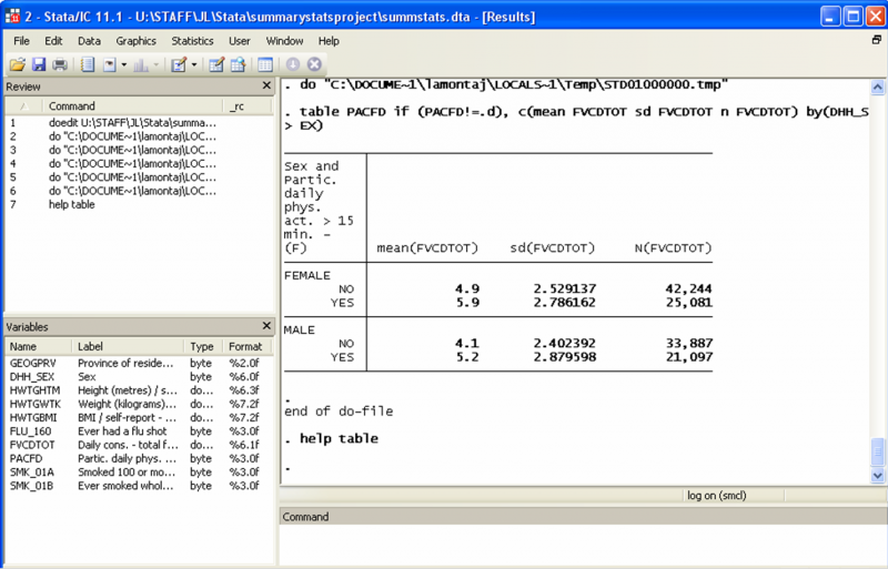
This will make a table with PACFD as the row variable (but only if the value for PACFD is not .d[5]), DHH_SEX as the superrow variable, and the content of each cell will be mean, standard deviation and frequency of the variable FVCDTOT:
Can we do better? Yes, we can. Up to four variables may be specified in the by(), so with the three row, column, and supercolumn variables, seven-way tables may be displayed. We won’t be doing a seven-way table today, but let’s look at a four-way table with superrow (a five-way table if you’d like):

The syntax is the same, it only looks more complicated.
table rowvar [colvar [supercolvar]] [if] [in] [weight] [, options][6]
In our example, the row variable is again PACDFD, the column variable is SMK_01B. We are using the if qualifier to restrict to observation for which the values of the row and column variables is either 0 or 1, the content of the cells is again mean, standard deviation and frequency of the variable FVCDTOT, and we have DHH_SEX as a superrow variable.

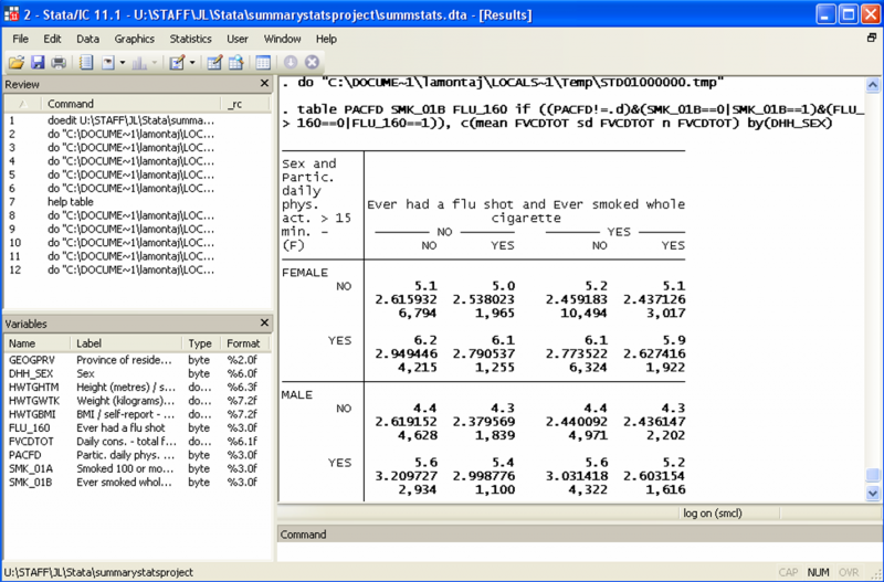
The way to read this table is simple: a female respondent who does not engage in more than 15 minutes of daily activity and has never smoked a whole cigarette eats on average 5.1 units of fruit and vegetables daily.
Now, a final flourish… A four-way table with supercolumn and superrow… Here is the command:
table PACFD SMK_01B FLU_160 if ((PACFD!=.d)&(SMK_01B==0|SMK_01B==1)&(FLU_160==0|FLU_160==1)), c(mean FVCDTOT sd FVCDTOT n FVCDTOT) by(DHH_SEX)
And the result:
Now, you may ask yourself, do I really need to do all that just to look at summary statistics? The answer will vary based on your level of sophistication, your research question, or your supervisor research agenda… For some, tabulate, summarize and maybe tabulate, summarize() will be more than enough. For others, tabstat and table might be very useful tools indeed.
We encourage you to play with data, and to gain an intimate knowledge of your dataset before conducting more formal statistical analysis. There are many good interenet sources for supplementary readings on creating summary statistics in Stata. Be specific when you enter a query in a search engine and you should find much user-written advice.
[1] Refer to guides on getting data from <odesi>, cleaning data on Stata
[2] You’ll notice a few administrative commands before the describe command (here shortened to “des”)
[3] The syntax would simply be: tab DHH_SEX if GEOGPRV==35, sum(FVCDTOT)
[4] We can’t draw inference from looking at means; we would need to test whether or not any of these means is statistically different from the others. However, looking at these summary statistics is a good start investigating patterns in the data.
[5] In this dataset, .d is a missing data code
[6] Type “help table” in the command window of Stata for a detailed presentation of the features of this command.