The main dataset used is the shelters dataset. It contains the Toronto daily shelter services from 2021 to 2026 [1]. Resources are listed below. If you need assistance, fill out the support request form.
TABLE OF CONTENTS
Importing Data
Exploring Data
Graphs
New Variables
Managing Data
Resources
Importing Data
Working directory
The directory is the place on your computer that is the home for R; therefore, this is where R is saving files and also where R is looking for files. Because R might be using a folder buried deep in your computer’s hard drive, there are two ways of finding and setting your working directory. First, you can use getwd() to find the current directory and setwd() to set the directory to a different path. NOTE: need to use the forward (/) instead of the backward slash (\) for directory paths in R.
getwd()
setwd("/Users/nadia/Desktop")
The second way is by going under File on the menu bar and going down to Change dir. This way is best if you do not know the exact name and location of where you want to set your new working directory because it allows you to go through all of the files on your computer.
Importing Data
DATA: shelters.csv
Download the shelters dataset by clicking on the link above or using the url uoft.me/shelterscsv.
Use read.csv() to read csv files. Set the header option to true if the file has column titles and false otherwise. The default option is always true.
shelters<-read.csv("Toronto Daily Shelter Overnight Occupancy 2021-2026.csv")
Exploring Data
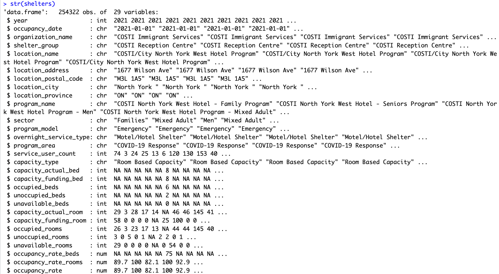
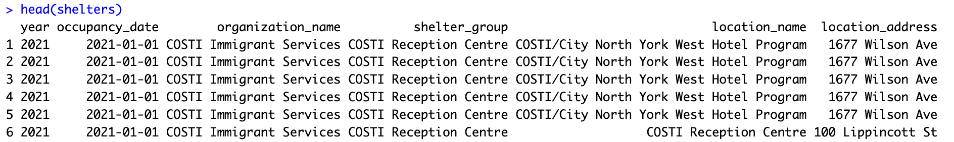
Unless you opened the .csv file beforehand, you don’t know much about the information you just loaded into R. To find out more, use the dim() function to find out the dimension of a data set. To view to contents of a dataset, use the str() function. The head() function displays the first six rows of the dataset and tail() displays the last six rows.
str(shelters)
head(shelters)
tail(shelters)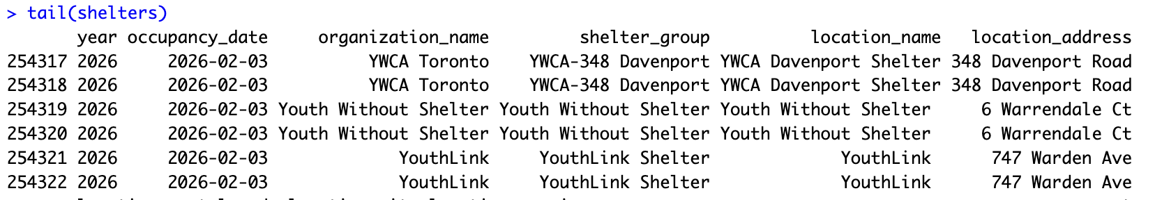
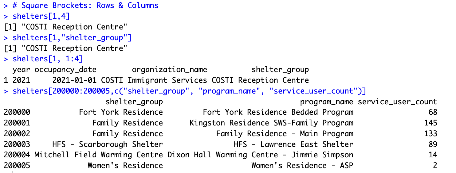
To open or, in R terminology, print the content of a data set or a variable in the R-console, simply write the data set or the variable. A data set has 2 dimensions. The first dimension is the row number and the second dimension is the column number. The two dimensions are separated by a comma. For example, shelters[1,7] prints the value in the first row and seventh column of the shelters dataset, shelters[1, ] prints the first row and shelters[,7] prints the seventh column. As you may notice, we use square brackets when isolating data and round brackets when working with functions. To print a range of rows or a range of columns, indicate the range separated by a colon.
shelters[1,4]
shelters[1,"shelter_group"]
shelters[1, 1:4]
shelters[200000:200005,c("shelter_group", "program_name", "service_user_count")]
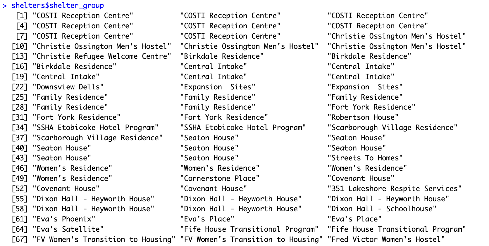
When we type a variable by itself, it gives us an error message. To access a variable, use the dollar sign “$”. For example, shelters$shelter_group returns the shelter_group variable.
shelter_group
shelters$shelter_group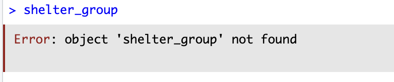
Frequency Tables
The table() function can be used to make a frequency table. You will also find functions from external packages that can be used to make frequency tables.
The table() function can be used to make a frequency table. You will also find functions from external packages that can be used to make frequency tables.
table(shelters$program_area)
table(shelters$program_area, useNA = "ifany")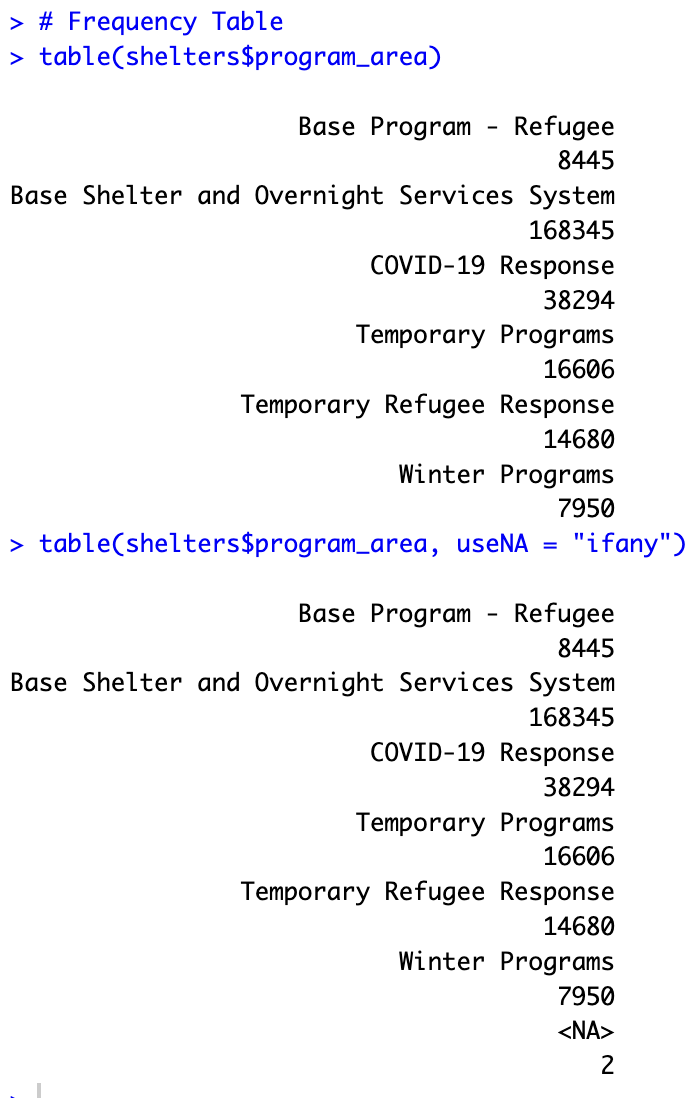
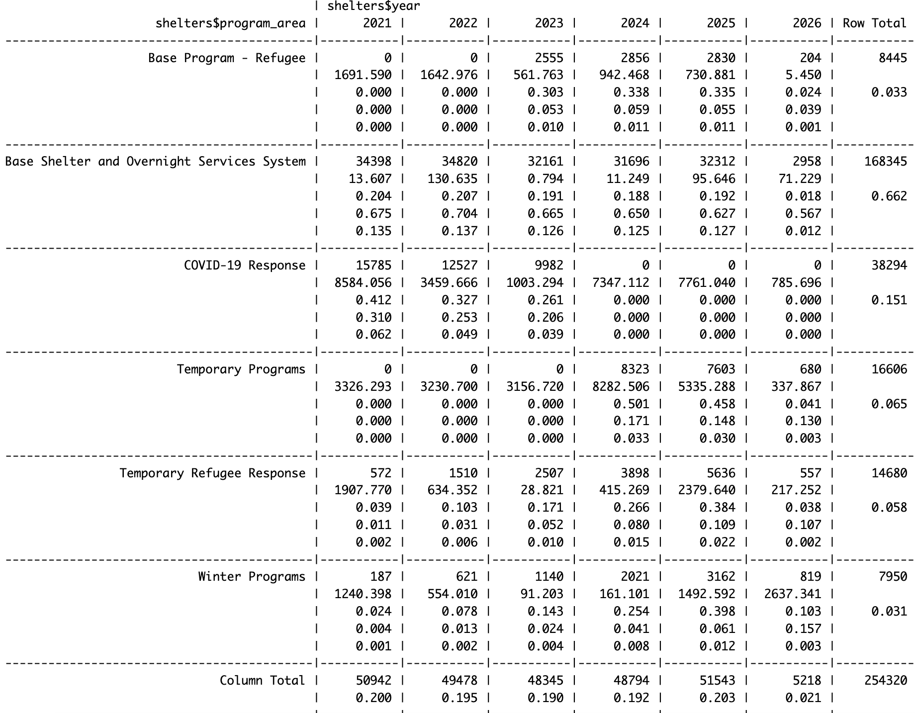
You can use the CrossTable() function from the gmodels package to make a two-way frequency table. First, you need to install the gmodels package using the install.packages() function and load it using the library() function.
install.packages("gmodels")
library(gmodels)
CrossTable(shelters$program_area, shelters$year
Descriptive Statistics
The summary() gives a summary of the object. If the object is a data set, it gives a summary of all the variables in a data set and if it is a variable, it gives a summary of the variable. Other descriptions can be obtained using the fivenum(), min(), mean(), max(), var(), quantile() functions.
summary(shelters)
summary(shelters$service_user_count)
mean(shelters$service_user_count, na.rm=TRUE)
sd(shelters$service_user_count, na.rm=TRUE)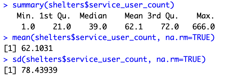
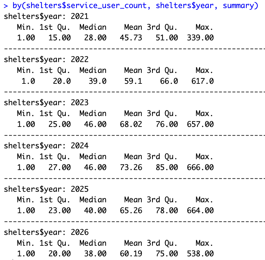
The by() function can be used to view the average shelter user count rates by another category. For example, below, we can see the average user count by year.
summary(shelters$service_user_count[shelters$year==2026])by(shelters$service_user_count, shelters$year, summary)
# Service_user_count grouped by organization
by(shelters$service_user_count, shelters$organization_name, summary)
# Alternative Approach to by()
aggregate(service_user_count ~ organization_name, data=shelters, summary)
Graphs
The following codes can be used to make bar charts, pie charts, boxplots and scatterplots. These are just a few of the many data visualizations you can produce using R. Each example shows you how to add more information to better develop the data visualization, so the below images are made using the last code in the entry.
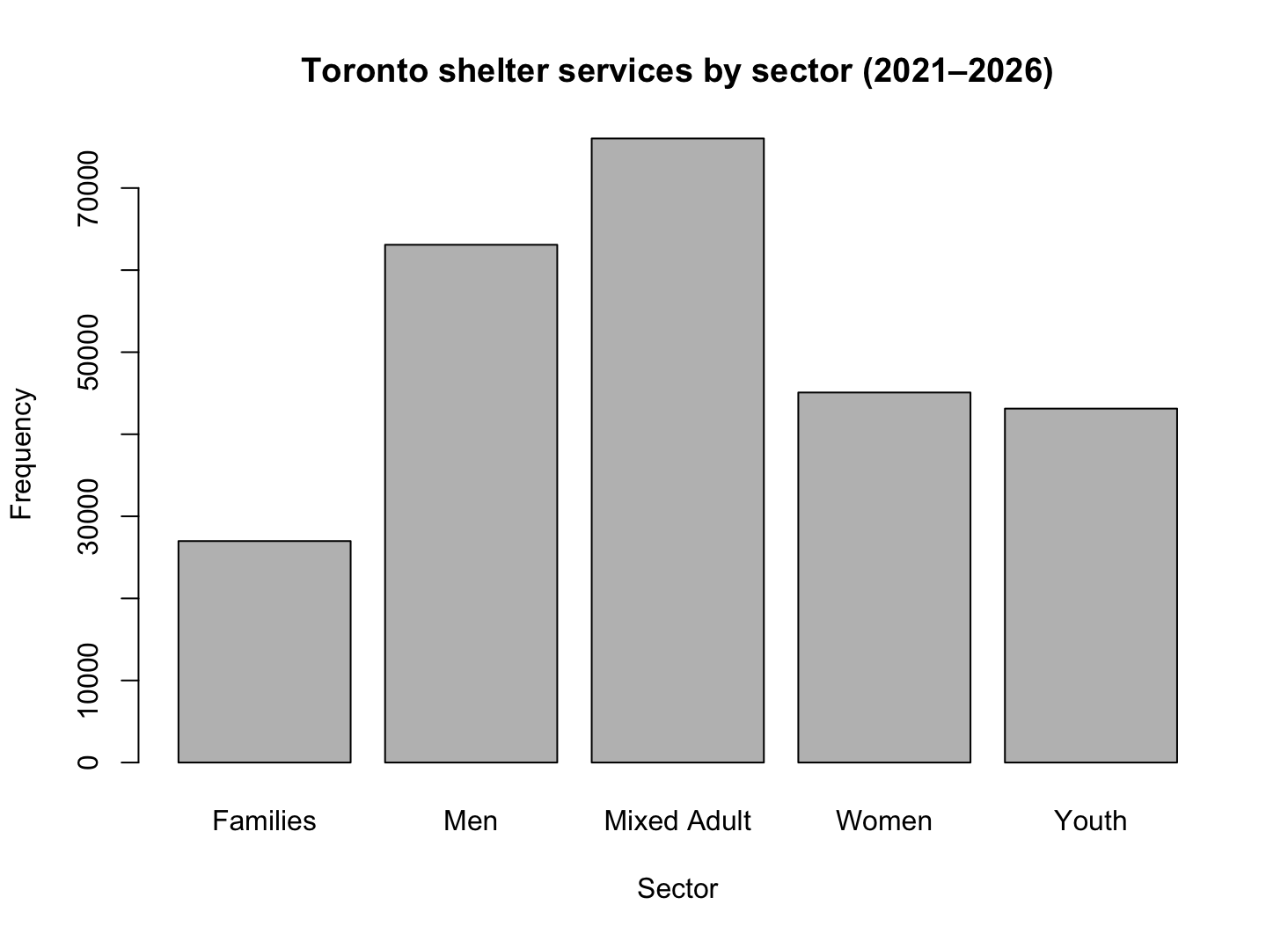
Bar chart
# Bar chart
shelterservicebysector <- table(shelters$sector)
barplot(shelterservicebysector,
       main = "Toronto shelter services by sector (2021–2026)",
       xlab = "Sector",
       ylab = "Frequency")
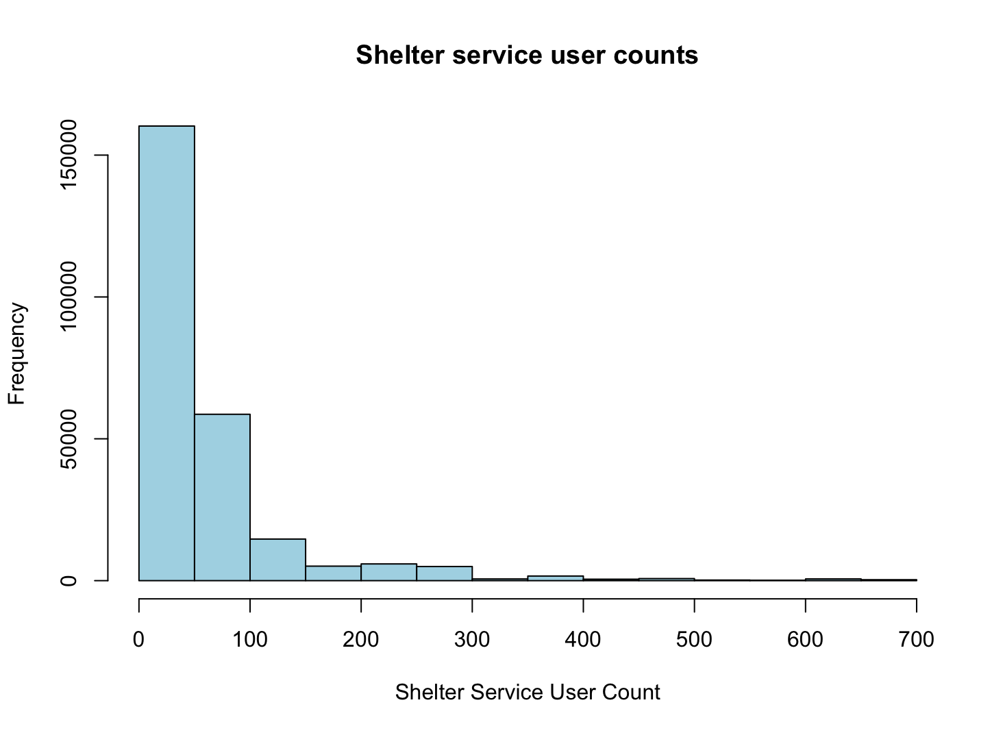
Histogram
# Histogram
hist(shelters$service_user_count,
    main = "Shelter service user counts",
    xlab = "Shelter Service User Count",
    col = "lightblue")
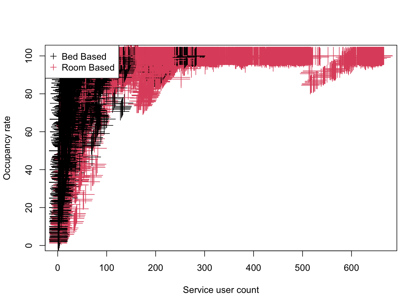
Scatterplot
# Scatterplot
plot(shelters$service_user_count, shelters$occupancy_rate)
plot(shelters$service_user_count, shelters$occupancy_rate, pch=3, cex=3, col="darkred")
plot(shelters$service_user_count, shelters$occupancy_rate,
    pch=3, cex=3, col=as.factor(shelters$capacity_type))

plot(shelters$service_user_count, shelters$occupancy_rate,
    pch = 3, cex = 3,
    col=as.factor(shelters$capacity_type),
    xlab = "Service user count",
    ylab = "Occupancy rate")

# Add legend to plots
legend("topleft", legend = c("Bed Based", "Room Based"), col = 1:2, pch = 3)
New Variables
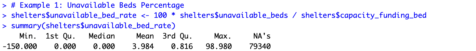
To generate a new variable that is a combination of other variables, assign the combination to a new variable name.
# Example 1: Unavailable Beds Percentage
shelters$unavailable_bed_rate <- 100 * shelters$unavailable_beds / shelters$capacity_funding_bed
summary(shelters$unavailable_bed_rate)

# Example 2: Youth Shelter Services Indicator
shelters$youth <- ifelse(shelters$sector=="Youth", 1, 0)
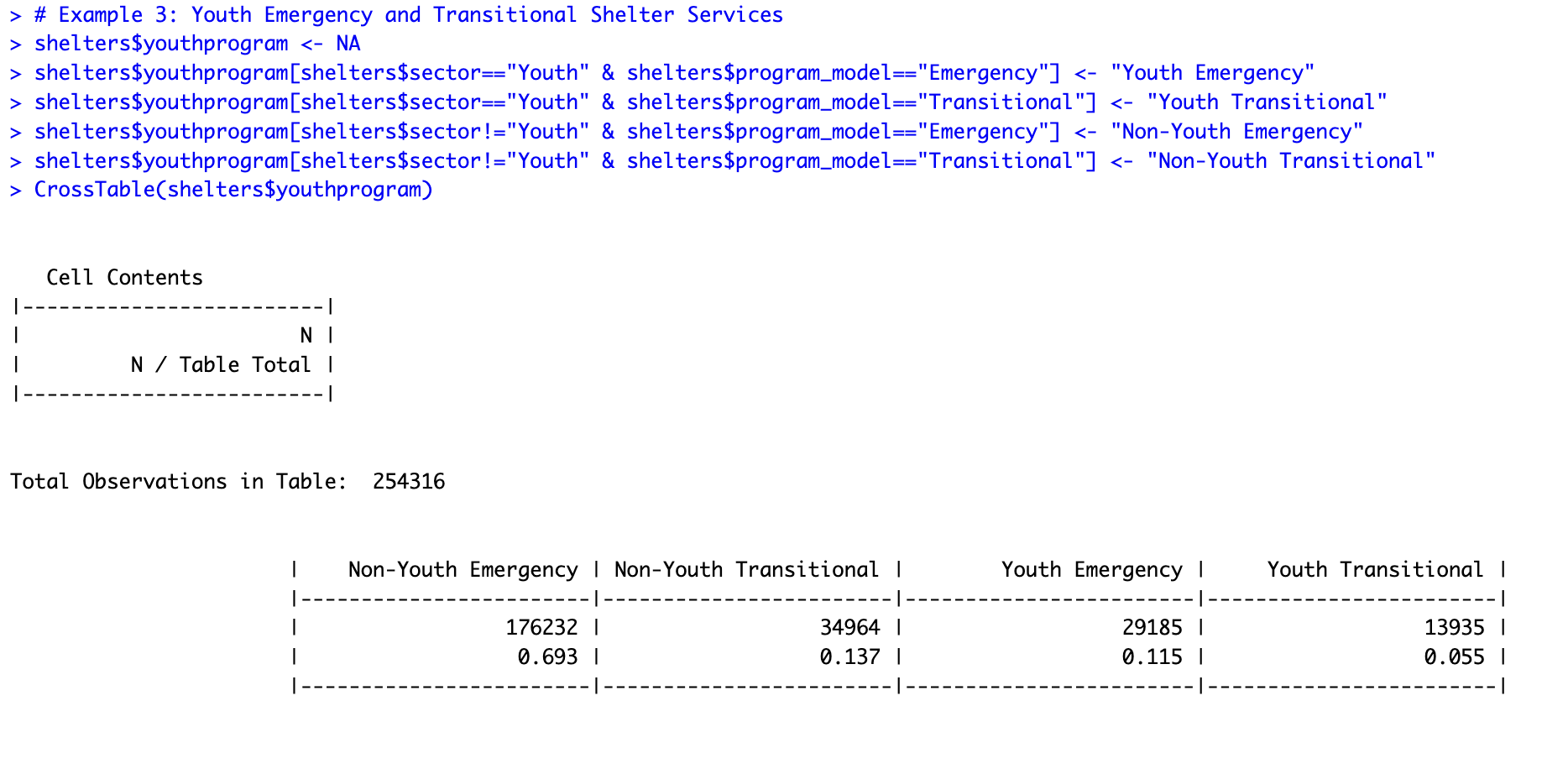
# Example 3: Youth Emergency and Transitional Shelter Services
shelters$youthprogram <- NA
shelters$youthprogram[shelters$sector=="Youth" & shelters$program_model=="Emergency"] <- "Youth Emergency"
shelters$youthprogram[shelters$sector=="Youth" & shelters$program_model=="Transitional"] <- "Youth Transitional"
shelters$youthprogram[shelters$sector!="Youth" & shelters$program_model=="Emergency"] <- "Non-Youth Emergency"
shelters$youthprogram[shelters$sector!="Youth" & shelters$program_model=="Transitional"] <- "Non-Youth Transitional"
CrossTable(shelters$youthprogram)
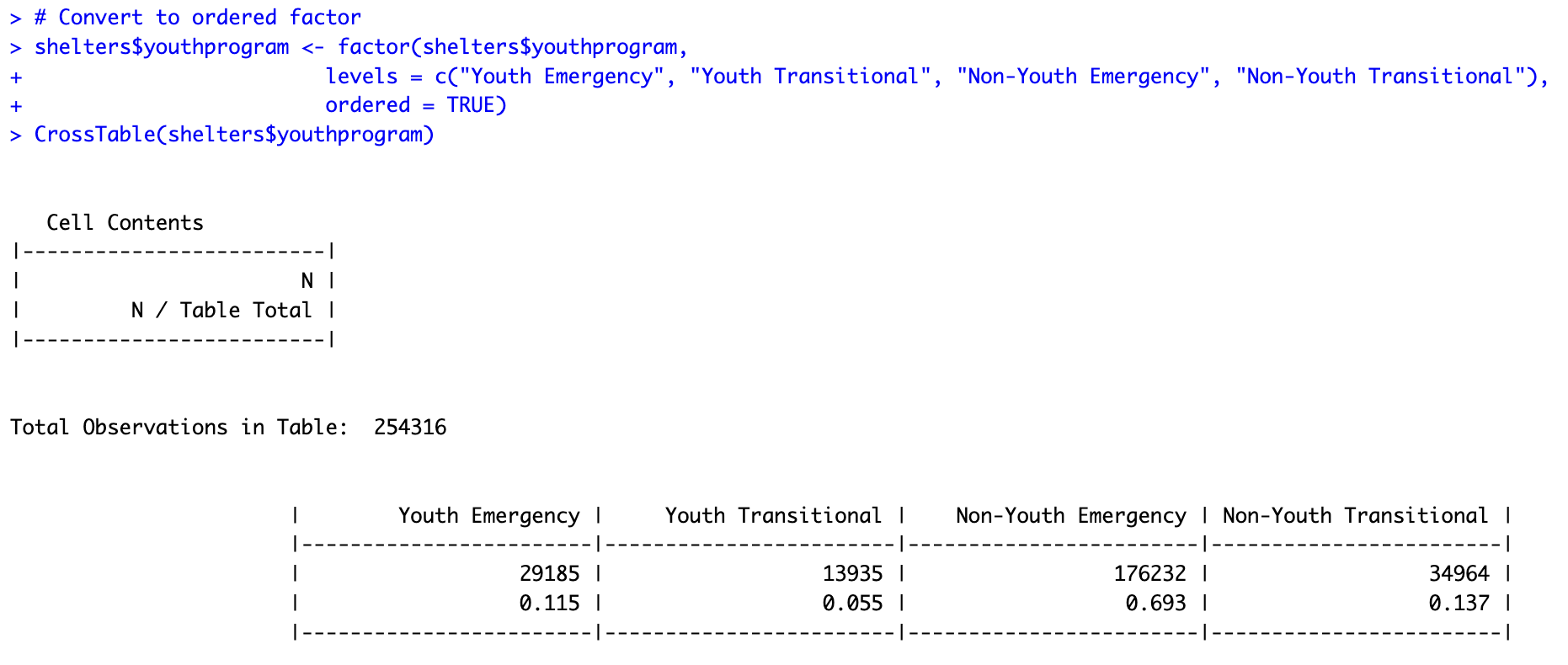
# Convert to ordered factor
shelters$youthprogram <- factor(shelters$youthprogram,
                       levels = c("Youth Emergency", "Youth Transitional", "Non-Youth Emergency", "Non-Youth Transitional"),
                       ordered = TRUE)
CrossTable(shelters$youthprogram)
save() can be used to save a dataset as a native R .RData data file.
# Saving Data
save(shelters, file="Toronto Shelter Services 2021-2026.RData")
# Exporting Data As CSV
write.csv(shelters, file="Toronto Shelter Services 2021-2026.csv", row.names=FALSE)
Managing Data
Subsetting Data
To subset, use the subset() function. You can subset by columns, conditions, or both.
To select a set of columns, you can use the select argument.
# Subsetting By Column
shelterprograms <- subset(shelters, select=c(year, organization_name, shelter_group, program_name))
To subset a dataset by a set of conditions, you can either enter the conditions as a second argument after entering the dataset or use the subset argument.
# Subsetting By Condition
youth2024_2026 <- subset(shelters, sector=="Youth" & year>=2024)
Resources
[1] The shelter dataset is modified from the original version on the Toronto Open Data portal.
[2] The tutorial code and the workshop Powerpoint presentation can be downloaded from here.
[3] You can enroll in the introductory R Quercus course here.