Cleaning data in STATA

Table of Contents

• Some useful tips before you get started
• Creating a number of smaller subsets based on research criteria
• Dropping observations
• Dropping variables
• Transforming variables
• Dealing with outliers
• Creating new variables
• Moving variables
• Labelling variables
• Renaming variables
• A few last words

 

Cleaning data is a rather broad term that applies to the preliminary manipulations on a dataset prior to analysis. It will very often be the first assignment of a research assistant and is the tedious part of any research project that makes us wish we HAD a research assistant. Stata is a good tool for cleaning and manipulating data, regardless of the software you intend to use for analysis. Your first pass at a dataset may involve any or all of the following:

• Creating a number of smaller subsets based on research criteria
• Dropping observations
• Dropping variables
• Transforming variables
• Dealing with outliers
• Creating new variables
• Moving variables
• Labeling variables
• Renaming variables

Whether this is your first time cleaning data or you are a seasoned “data monkey”, you might find some useful tips by reading more.

Some useful tips before you get started[1]

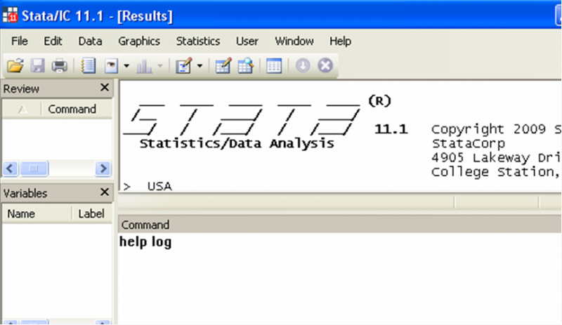
Use the Stata help file. Stata has a built in feature that allows you to access the user manual as well as help files on any given command. Simply type “help” in the command window, followed by the name of the command you need help with and press the Enter key:

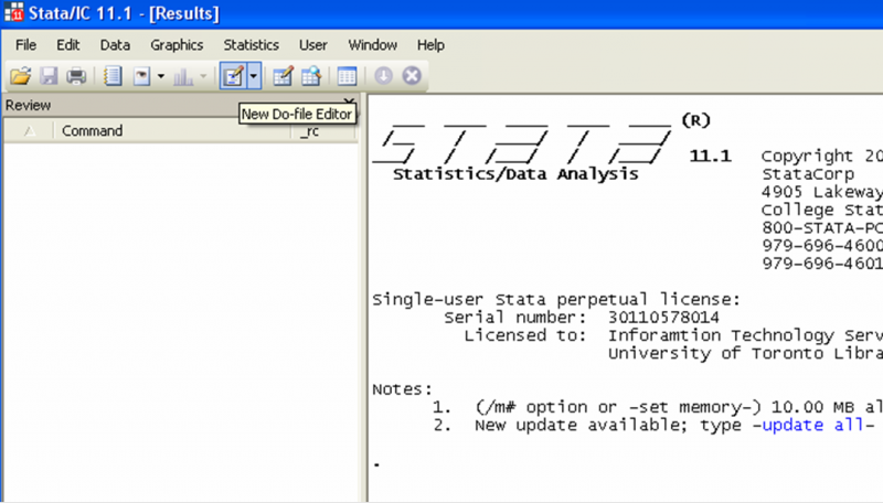
Write a do file. Never clean a dataset by blindly entering commands (or worse, clicking buttons). You want to write the commands in a do-file, and then run it. This way, if you make a mistake, you will not have ruined your entire dataset and you will not need to start again from scratch. This is a general advice that applies to any work you do on Stata. Working from do-files lets other people see what you did if you ever need advice, it makes your work reproducible and it allows you to correct small mistakes somewhat painlessly. 

To start a do-file, click on the icon that looks like a notepad on the top-left corner of your Stata viewer[2].

In the preliminary stages of your work, you may feel that a do-file is more hindrance than it is useful. For example, if you are not so familiar with a command, you may prefer to try it first. One simple way to do that and still have discipline about writing do-files is to write your do-file in stages, writing only a few commands before executing them, correcting mistakes as you go. In order to execute a number of commands rather than the whole do-file, simply highlight the ones you want to execute, and click on the “Execute Selection (do)” icon on the top of your do-file editor, at the far right.

As you become more proficient with programming in Stata, you won’t need to try out commands anymore, and you’ll discover the joy of writing a do-file and having it run without a glitch. To run a whole do-file, do not highlight any part of it and click on the “Execute Selection (do)” icon.

You may wonder about the commands “clear”, “set more off” and “set mem 15000” in the screenshot example. These three commands are administrative commands that are quite useful to have at the beginning of a do-file. The first, “clear”, is used to clear any previous dataset you may have been working on. The command “set more off” tells Stata not to pause or display the --more-- message. Finally, the command “set mem 15000” increases the memory available to Stata from your computer; here we will need it as the size of the data set we downloaded from <odesi>[3] is larger than the 10mb allocated to data by default.

One last comment about do files: if you double click a saved do file, it will not open for editing, but rather Stata will run that do-file, which can be a bit annoying… To reopen a do-file from a folder without executing the commands in it, right-click on it and select “edit” rather than “open”.

Always keep a log. Again, this is a general rule of thumb on Stata. Keeping a log means you can go back and look at what you did without having to do it again. Starting a log is just a matter of adding a command at the top of your do-file that tells Stata to log, as well as where you want the log to be saved:

log using “whateverpathyouwant:\pickanameforyourlog.smcl”[4], replace[5]

Note how logs are saved under the smcl extension.

Do not forget to close your log before starting a new one. The last command on your do-file[6] will usually be “log close”.

Save as you go. Computers crash, power goes out, stuff happens. Save your do-files every few minutes as you write them. Saving a do file is done the same way as saving any text editor document: either click on the diskette icon, or press “CTRL+S”:  

You should also save your dataset as you modify it, but make sure to keep one version of the original dataset, in case you need to start over. The command to save a dataset on Stata is “save”, followed by the path where you want the dataset to be saved, and the [optional] command “replace”.

Note how the extension for Stata data is “.dta”, and also note how the new dataset has a different name from the original[7].

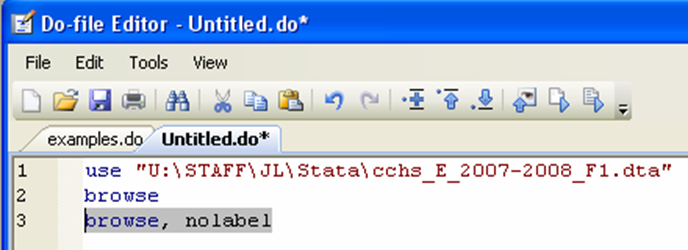
Become familiar with your dataset. Datasets come with codebooks. You should know what each variable is, how it’s coded, how missing values are identified. A good practice is to actually look at the data, so that you understand the structure of the information. To do so, you can click on “Data” in the top-left corner of your viewer and select Data editor, then Data editor (browse). A new window will open and you can see your data.

You can also use the command “browse”, either by typing it directly in the command window, or from a do file:

One of the distinguishing features of <odesi> is that when you download a dataset, it comes with labels. Variable labels are descriptions of variables, and value labels are used to describe the way variables are coded. Basically, the value label sits on top of the code, so that when you browse, you see what the code means rather than what it is. To make this clearer, let’s look at the data with no labels. Look, for example, at the GEOPRV variable.

Back to top

Creating a number of smaller subsets based on research criteria

There are many reasons why you may want a smaller subset of your data but the main one is that the bigger the dataset, the harder it is for Stata to manage, which slows down your system. Your goal is to make your dataset as small as possible, while keeping all the relevant information. Your research agenda determines what your final dataset will contain.

Let’s say you have data on the health habits of Canadians aged 12 and up, but your research question is specific to women of reproductive age living in Ontario[8]. You clearly don’t need to keep the men in your dataset, and you won’t need to keep the residents of provinces other than Ontario. Furthermore, you can probably drop women under 15 and over 55 years old. Now, let’s look at how you would do that.

Back to top

Dropping observations

To drop observations, you need to combine one of two Stata commands (keep or drop) with the “if” qualifier.

Make sure you have saved your original dataset before you get started.

The “keep” command should be used with caution (or avoided altogether) because it will drop all but what you specifically keep. This can be a problem if you are not 100% certain of what you want to keep.

The “drop” command will drop from your dataset what you specifically ask Stata to drop.

The “if” qualifier restricts the scope of the command to those observations for which the value of an expression is true. The syntax for using this qualifier is quite simple:

command if exp

Where command in this case would be, drop and exp is the expression that needs to be true for the “drop” command to apply[9].

Using the example of women of reproductive age in Ontario, the first highlighted line drops men, the second line drops any observation not in Ontario, while the last line drops observations in age groups older or younger than our subset of interest.

You have to be careful with logical operators; notice the syntax in the third line. A common mistake is to ask Stata to “drop if DHHGAGE>10&DHHGAGE<2”. There are no individuals in the dataset who are older than 55 AND younger than 15. We want to drop if older than 55 OR younger than 15.

Here is a list of operators in expressions. You would mostly use logical and relational operators in conjunction with “if”:

Back to top

Dropping variables

Another way in which you may need to make your dataset smaller is by dropping variables that are not useful to your research. It may be that the information contained in a given variable is duplicated (i.e. another variable provides the same info), or maybe all the observations for a variable are missing, or a variable just happens to be in your dataset but is irrelevant to your research. Dropping variables is very straightforward; simply use the “drop” command.

Looking at the data from CCHS, the variable SLP_01 (Number of hours spent sleeping per night) is coded as “.a” (NOT APPLICABLE) for each observation in the dataset.

Clearly we will not learn anything from that variable, so we can drop it. The syntax for dropping variable is simple:

drop varlist

Where varlist is the list of variables you would like to drop. It’s easy to drop a number of a variable at a time this way. Here I am dropping all the variables that were coded as Not Applicable for more than 95% of observations[10]:

Back to top

Transforming variables

Sometimes variables are not coded the way you want them to be. In this section we will look at two transformations you may need to do on some variables before using them: recode and destring.

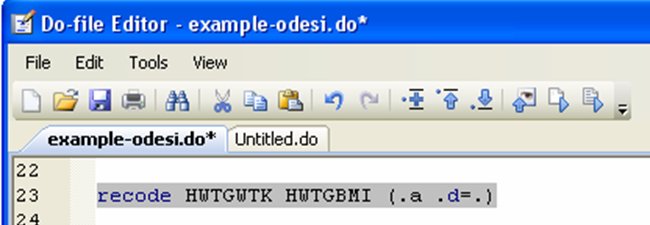
The “recode” command changes the values of numeric variables according to the rules specified. In the CCHS dataset, many variables have missing values coded as “.a” or “.d”. This is convenient because it will not affect calculations you might do using the data (for example if you calculate an average). However, many datasets use 999 as a missing variable code, and that might be problematic. We might want to recode these as “.” in order to not have them affect any calculations we plan on doing with the data. The syntax for this command is:

recode varlist (old value(s)=new value)[11]

Let’s recode the height and BMI variables from the CCHS data, (for the sake of illustration, since it’s really not necessary in this case):

The “destring” command allows you to convert data saved in the string format (i.e. alphanumeric) into a numerical format. The CCHS dataset does not contain any string variable. In order to see what a string variable looks like, we can use the converse command, “tostring”, to create a string variable. We will then convert that variable back to a numerical format.

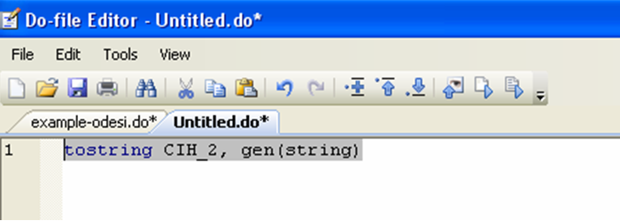
A string variable shows up in red in the data editor:

Although it may look the same as the variable CIH_2, Stata cannot do any calculations on the string variable (since its format is telling Stata that it is made of letters or other symbols). Let’s destring it:

Notice the use of the options “generate” and “replace”. When we created the fake string variable, we used “generate” because we wanted a new separate variable. Now, when we destring, we are replacing the string variable by its numerical counterpart. How you choose to do this in your own dataset depends on how you plan to use the variables. Will you still have any use for the string variable? If so generate a new one when you destring. Do you just want that variable to not be in string format? Then replace it with the new one. 

Here, we can see that our variable string is now completely identical to the variable CIH_2:

(We can drop that variable now)

Back to top

Dealing with outliers

Outliers deserve their own section because there is often confusion as to what exactly constitutes an outlier. An outlier is NOT an observation with an unusual but possible value for a variable[12]; rare events do occur. The outliers you should be concerned about are the ones that come from coding error. How do you tell which is which? Common sense goes a long way here.

First, look at your data using the data editor (browse). Outliers tend to jump at you. If you have a small dataset, you can also tabulate each of your variables:

tab varlist[13]

Tabulating a variable will give you a list of all the possible values that variable takes in the dataset. Outliers will be the extreme values. Look at the order of magnitude. Are these values believable?

If the dataset is very big, however, it may not be practical to stare at all the values a variable can take. In fact, Stata will not tabulate if there are too many different values. 

You can look at your data in a scatter plot:

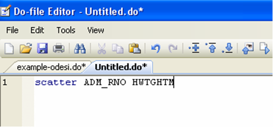
In the CCHS dataset, caseid is the individual id, while hwtghtm is the height in meters. The graph tells us there are no outliers in this dataset:

Another way to look for outliers is to summarize the observations for a variable, using the detailed option:

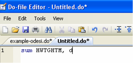
The result window will show the main percentiles of the distribution (including the median – 50%), the first four moments, as well as the four smallest and four largest observations:

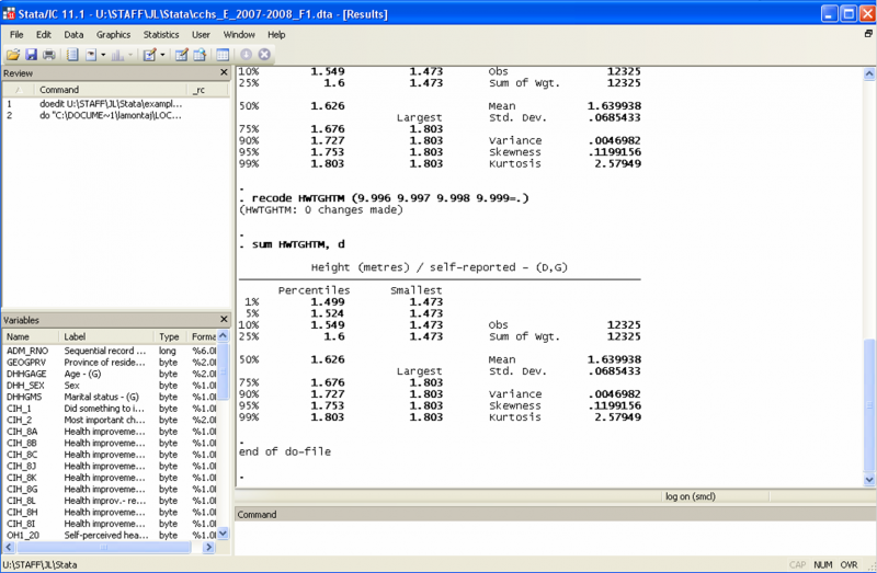
Clearly, there are no outliers. Let’s imagine for a moment that the 99 percentile of the height distribution includes an observation with 5.2m entered as the height. Is it plausible that there really was a 5.2m woman recorded in this dataset? Look at the order of magnitude by which this observation would differ from the second largest. It’s almost 50 standard deviations bigger...

What should you do with such an observation? There are a number of solutions but none is perfect:

• Drop it from your dataset (“drop if hwtghtm>1.803”)
• Use the “if” qualifier to exclude it when generating statistics that use the height variable (“command if hwtghtm<=1.803”)
• Ignore it if the height variable is not actually that important in your research and the rest of the variables for this observations are coded just fine

Back to top

Creating new variables

There are two main commands you need to know to generate new variables: “gen” is for the basics, while “egen” allows you to get pretty fancy. You can combine these with qualifiers such as “if” or “in” as well as prefix such as “by” and “bysort”[14].

For example, say you want to create a variable that tells you whether the women in the dataset have a live-in partner. While there is no sure-fire way to establish that, we will approximate it by assuming that women who indicated their marital status as married or common-law actually live with their spouse or common-law partner:

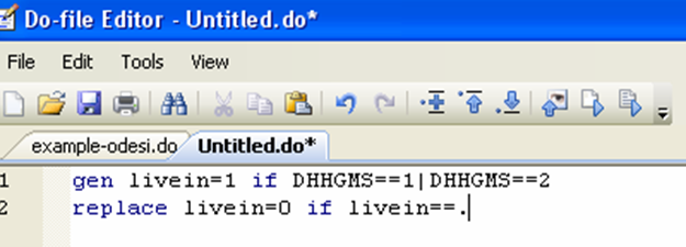
The first line creates the variable “livein” and assigns it a value of 1 if the value of the marital status variable (dhhgms) is either 1 (married) or 2 (common-law). The second line replaces the missing value code by 0, making the “livein” variable binary.

Now, let’s say you would like to create a categorical variable that tells you, by age group, if a woman is below or above average in terms of body mass index (BMI).

The first line of command creates a variable (meanbmi) which takes on a unique value for each age group, the average BMI for that age group. The prefix “bysort” is a combination of “by” and “sort”; you could equivalently break it into two commands:

sort DHHGAGE

by DHHGAGE: egen meanbmi=mean(HWTGBMI)

The “sort” part of the command organizes the observation according to the variable DHHGAGE, from smallest to largest, a step required before doing any action “by” the variable. It’s usually easier to just use “bysort”.

The second and third lines (starting with “gen”) create a binary variable which equals 0 if an observation has a BMI lower than the average for her age group, and 1 if her BMI is above her age group average. 

Back to top

Moving variables

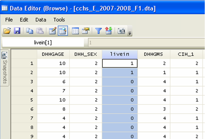
Now that you have created these new variables, it would be nice to make sure that the rules by which you generated them was correct. Ideally, you would like to look at livein (the new variable based on marital status) and dhhgms (the marital status variable). However, it’s hard to compare two variables unless they are side by side. You can use the “order” command to move a variable (i.e. move a column of your dataset).

When you create a variable, by default it becomes the last column of your dataset. You can move it next to another variable instead:

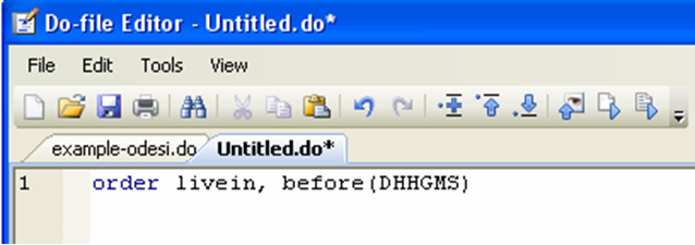
Now if we look at our dataset, we can see compare the new variable to the old and make sure that we coded it properly:

Similarly, since our two new variables pertaining to BMI are now the last columns, let’s move the original BMI variable to the end of the dataset:

It now easy to glance at our new variables:

Do you notice the problem on line 8? The variable bmicat should not be coded 1 if the original BMI variable is coded as a missing value. We can fix this with a quick replace:

replace bmicat=. if hwtgbmi==.d

Back to top

Labelling variables

Whenever you create a new variable, it is a good idea to label it. Why? Having your variables labeled makes it easy for you or anyone else using your dataset to quickly see what each variable represents. You should think of your work as something that people should be able to reproduce. Labeling your variables is a small task that makes it much easier for others to use your data[15].

The syntax for labeling variables is as follow:

label variable varname “label”.

In our previous example, the command would look like this:

Note that you can abbreviate this command to lab var:

Back to top

Renaming variables

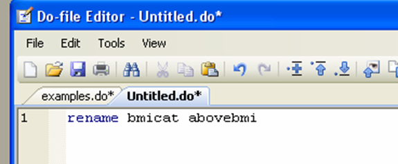
You may find that you work faster if your variables have names that you recognize at first glance. In most cases this is by no means a necessary task in cleaning data, but if you use data from another country, for example, you may find that the variable names are in a foreign language, making it very hard to remember. The syntax is as easy as can be:

rename oldname newname

Let’s see the final do-file

Your do-file may be slightly different from this but it should result in the same final dataset:

Let’s try running it in one go to see if it works. Do not highlight any command and click on Execute (Do). Note that whenever Stata encounters the command “browse” a data editor will pop up on your screen. Have a look at your data then close the data editor in order for Stata to continue running the do-file.

Let’s also take the time to open our logs to see what it looks like and how it could be useful.

Finally let’s look at our final datasets and make sure it contains all the right variables, in the right format.

Back to top

A few last words

This concludes our workshop but it’s only the beginning for you. Learning to use statistical software involves a lot of trial and error, angry googling, and desperately trying to find someone who knows how to write a loop… Listed below are a few excellent resources to further your working knowledge of Stata:

UCLA: http://www.ats.ucla.edu.myaccess.library.utoronto.ca/stat/stata/default.htm

 

Princeton: http://data.princeton.edu.myaccess.library.utoronto.ca/stata/default.html

http://www.princeton.edu.myaccess.library.utoronto.ca/~otorres/Stata/statnotes

 

LSE: http://personal.lse.ac.uk.myaccess.library.utoronto.ca/lembcke/ecStata/2009/MResStataNotesJan2009PartA.pdf

http://personal.lse.ac.uk.myaccess.library.utoronto.ca/lembcke/ecStata/2009/MResStataNotesFeb2009PartB.pdf

 

University of North Carolina at Chapel Hill: http://www.cpc.unc.edu.myaccess.library.utoronto.ca/research/tools/data_analysis/statatutorial

 

Stata: http://www.stata.com/support/faqs/

Back to top