Before you begin, make sure you have NVivo 12 installed. If you don’t, follow these instructions to request a free license key and install the software.
You’ll also need to download some datasets that we’ve provided for this tutorial. Create a new folder on your computer to store the tutorial files. Download this zip file containing all the datasets you will need for the tutorial to that new folder. Finally, extract the files into that new folder.
This tutorial is adapted from a recorded NVivo 12 workshop, which you can view here.
Table of Contents
Creating a New Project
Explore the Interface
Import Data
Creating Nodes and Coding
Working with Nodes
Creating Notes
Case Classification and Cases
Save the Project
Word Frequency and Text Queries
Coding Queries
Matrix Coding and Crosstab Queries
Export Data
Resources to Learn More
Test your Understanding Answers
Part 1 – The Basics
Creating a New Project
1. First start up NVivo 12. From the main screen you can start a new project, open some sample projects, and access several resources for learning and using NVivo. We will look at a sample project later. For now, click on Blank Project to get started.

2. Title your project. For this tutorial we will name ours “NVivo Workshop”. If you’d like, you can add a description.

3. Next, browse to where you want to save the project file. Let’s save it in our workshop folder.

4. Check the “Write user actions to project event log” option. This will record everything you do in NVivo in a log file. If you have any issues and contact QSR for help, their customer service representatives might ask you for this log file, as it will help them troubleshoot your problems.

5. Finally select OK to create your new project.
Explore the Interface
1. Let’s briefly look around before we get started. First off, NVivo will present you with a getting started tutorial video. You can just close that tab for now.
2. The left side menu helps you navigate the various items of your project, such as your files, themes, notes, queries, etc. We will look at these sections as we use the tool.

3. At the top are various ribbon menus, similar to Microsoft tools, such as Word or Excel. These menus and their options will change depending on what is selected.
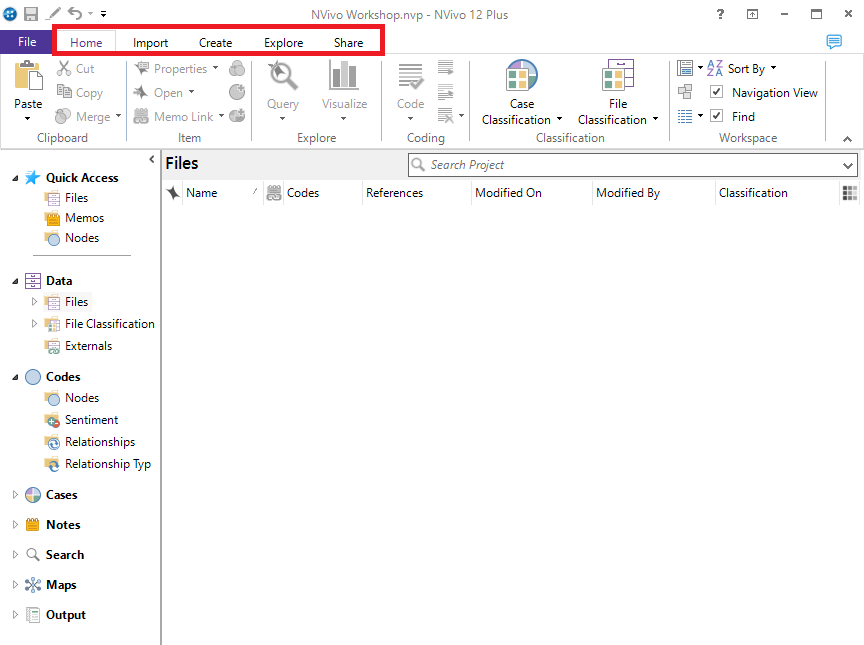
4. NVivo will ask you to save your project every 15 minutes. But if you want to save it manually, create or open a new project, get help or change your program settings, you can use the File menu at the top left.

5. If you select File, and then Help, you will see an option for Manage License, where you can update your license key, when you receive a new one each year.

6. Click on the top left arrow to get back to NVivo’s main screen.

Import Data
Next, let’s import some data so we can start using the tool. We will be using transcripts from interviews and focus groups run for a US data center study. As mentioned before, NVivo helps you get organized, so before we import in some data, let’s create some folders to organize our data.
1. From the left menu, expand Data, then right click on Files and select New Folder. Call it “Interviews”.


2. Create another folder called “Focus Groups”.

3. Next, select the Import ribbon at the top left. Here you can see all the various types of files that NVivo can import.

4. To start, let’s import in our interview transcripts. Make sure that the Interviews folder is selected on the left. Then select Files from the Import Ribbon.

5. Browse to the folder called “DCEE Focus Groups and Interviews,” which has all the study files we will use in this tutorial.

6. If you select the Supported Formats drop-down menu at the bottom right of the pop-up window, you will see all the different file types that you can import into NVivo. In our case, we are starting with .docx files (i.e., MS Word files), so make sure to select Document Files.

7. Highlight only the files starting with “Data Center Interview” in the title in our folder by selecting the first one, holding down the Shift key, and then selecting the last one. You should have 7 files highlighted. Then select Open.

8. Select Import to import those interview transcripts into the Interviews folder. Ignore the “Create a case” option for now. We will discuss it later.

9. Let’s do something similar to import in the focus group information. Select the Focus Groups folder on the left. Then select Files from the Import ribbon.

10. You should still be in the same folder when you select Browse. This time highlight the files with “FG” in the title. You should have 8 files. Keep the default, Supported Files selected. This will allow you to import a combination of word files and PDFs in one go. Then select Open.

11. Then select Import to import those focus groups files to the Focus Groups folder.

12. These files are now all copied into your project file. You can see from the Import ribbon that there are many different file types that can be imported. For example, you can connect to survey tools or reference managers to pull in your data, or import in audio files, images, or videos. We won’t be covering them all in this tutorial, but be sure to explore your options later.

Note: If you’re interested in learning more about importing other common data sources into NVivo, check out our tutorial on importing webpages as PDFs and survey data!
Creating Nodes and Coding
One of the main tasks NVivo is used for is coding. NVivo has a Codes section from the left menu, but if you expand it, you will see folders such as Nodes, Sentiment, etc. NVivo calls your codes or themes “Nodes.” These nodes act like containers to hold all the references to that theme.
If you have already decided upon codes ahead of time (following a deductive approach to coding), you can add these codes to NVivo and then start using them. Other times, as mentioned, you will be reading your materials in NVivo and creating codes as you go (an inductive approach to coding). And sometimes you will do a combination of this, where you have a rough idea of some themes you expect to see, but then new themes might emerge for you as your read through the materials. For this example, let’s try this combo method. First, we will create a few nodes that we will use to code our materials, and then I will show you how to create nodes on the fly as you are reading.
1. From the Codes section on the left, right click on the Nodes folder and select New Node.

2. Alternatively, you can go to the Create ribbon and select Node to create a new node.

3. For the node name call it “Budget”.

4. You can add a description for your nodes if you like. This lets you describe them in more detail and give examples of where it would be applied to understand how to use it in coding. We will just leave it blank for now. The nickname field is used if your node name is a bit longer, but you want a quick nickname to select from a list when coding. Our node name is short, so we don’t need a nickname in this case. Ignore the “Aggregate coding from children” option for now. We will discuss it later. So let’s just select OK. You should now see our new Budget node listed in the Nodes folder.

5. Repeat the last three steps to also create a node called “Maintenance.” If you make a mistake, you can always right click on a node and select Delete to remove it (be careful with this option if you have started coding!) or select Node Properties to rename it or add a description and nickname. You should now have two nodes.

6. Now that we have a couple nodes, let’s use them to do some coding. To open up one of our imported files, from the left menu, go to the Interview folder under Files and double click on the first interview transcript to open it in NVivo.

Note: NVivo can open a lot of different file types directly in the tool. The files will be open as read-only, meaning you can’t edit them. This is intentional to prevent error. However, if you happen to notice an error you want to correct, you can select Click to Edit at the top of the file. Then you will be able to make changes to the file and save them.
7. With the file open, you can then read through it and code. Highlight some text you want to code, and then right click and select Code.

8. Next, select the node you want to use to code this text, such as Budget, and then click OK. Now it is coded.

Note: Generally, you want the text to match the coding category, but for now, don’t worry if the text doesn’t match, this is just to quickly show you how it works.
9. Let’s look at an alternative quick way to code. This time before you code, click on the Nodes folder. This should open up the Nodes list next to your transcript.
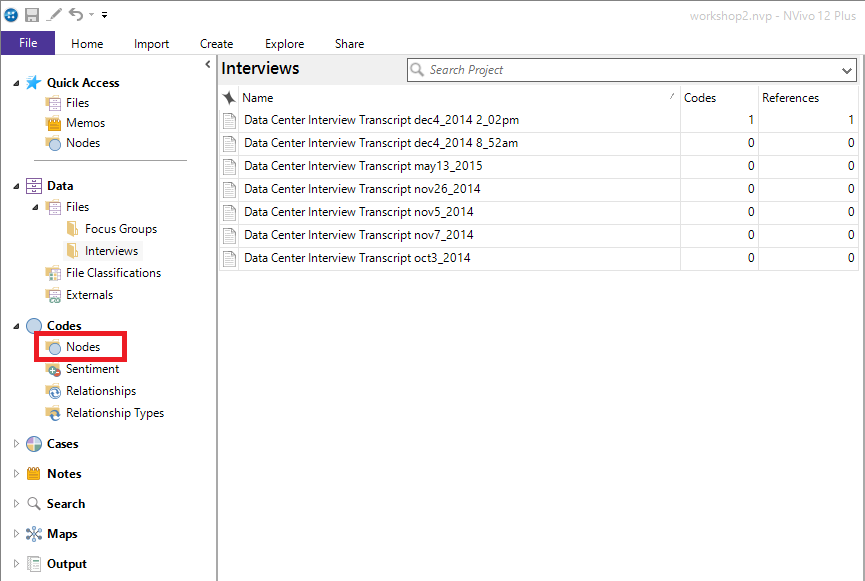
10. Highlight some text you want to code, and then drag the highlighted text over to the node you want to code it to. Let’s drag it over to the Maintenance node. This is a fast and visual way to code that lets you can see the full list of codes while you are coding.

11. So far we have been coding using our pre-made nodes. However, sometimes, something unexpected might come up that you want to create a new node to code it. Highlight some text, and then right click and select Code.

12. Now, instead of selecting an existing node, select New Node at the bottom left.

13. Here you can give it a name, for example, “Teamwork” and select OK to create a new node on the fly.

14. So far we have been coding Word documents, but let’s look at the PDFs we imported as well. First close the current interview transcript you have been working with.

15. Go to the Focus Groups folder and open up “NYC Data Center FG1 Questionnaire 7.”

16. This PDF file has been OCR’ed, meaning you can select text and code it as we have done before. Try selecting some text.

17. Now open up “NYC Data Center FG1 Questionnaire 14.”

18. This PDF file has not been OCR’ed, meaning you can’t select the text and code it as we have done before. Instead NVivo treats this more like an image. Select Region from the PDF Tools Menu at the top.

19. You will then be able to code this part as normal by right clicking and selecting Code. Generally, though, it is better to make sure that any PDFs you import into NVivo are OCR’ed for ease of coding. This will also be important when running queries, which we will look at later. For now, close these two PDFs.

Note: If OCR’ing PDFs is new to you, this guide might help.
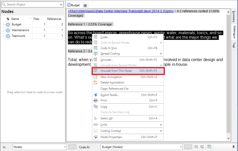
20. Go to the Nodes folder and double click on a node that has some references (meaning it has been used to code some text). Here you will see all the snippets of text that were coded to this node.

21. If you later realize that you mistakenly coded something you didn’t mean to code, you can uncode it. Highlight one of the references listed, and then right click and select Uncode from this node.
Working with Nodes
1. Before we work some more with Nodes, create two more nodes called “Energy Efficiency” and “Water Consumption”.
2. Next, code at least 5 small text fragments to each new node.
3. You can see now there are useful counts associated with our nodes to see how many files have content that has been coded in that node, and how many text snippets or references have been coded into that node.

4. You will notice that all of our nodes are top-level or parent nodes, meaning we haven’t established a hierarchy, none of our nodes are nested under other nodes. NVivo can help you organize your nodes in a hierarchical structure. You are often, in the end, trying to create a hierarchical nodes list to group common themes together into broader themes to help make sense of your coding. Create a new node and call it Sustainability.


5. You could use this node to thematically group some of your existing nodes. Drag Energy Efficiency and Water Consumption onto the Sustainability node (First click on a node to highlight, wait a moment, then drag it on).

6. Now you can see that they are grouped beneath. Nodes grouped beneath another node are called Child Nodes.

7. You can use Sustainability as its own broader node now in coding, or just keep it as a heading in the hierarchy. Double click on Sustainability. You should see an empty window pop up as there are no references coded to that node right now.

8. Right click on Sustainability and select Node Properties.

9. Click the box next to Aggregate Coding from children. Then click OK.

10. Now you should see all the references to Sustainability’s node, plus its children nodes, show up in the window that popped-up before (and is still open). You will need to decide how to want to handle your node hierarchies in terms of this aggregation for your own projects. In some cases, this is very useful, but it may affect queries where references are double counted for the parent and the child. We will talk more about queries later in the tutorial.

11. In the window with all the Sustainability references, highlight all the text. A quick way to do this is to click anywhere in that window and press CTRL and “A” on your keyboard at the same time to select all.

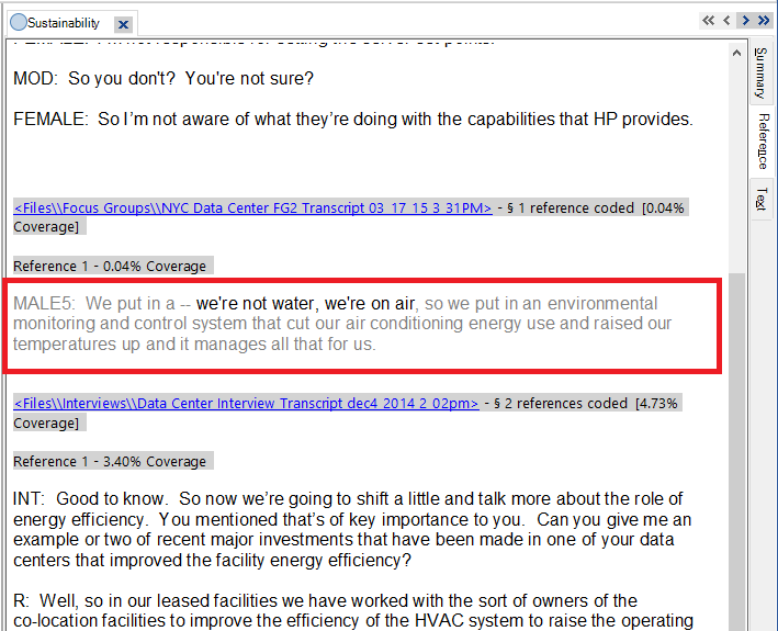
12. Then go to the Node ribbon menu at the top, select the Content drop-down menu and pick Broad under Coding Context.
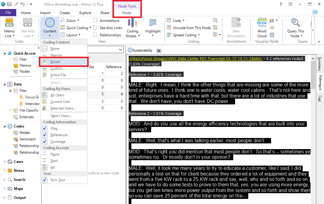
13. You will see that the references have changed. There is grey text that isn’t coded, but comes directly before or after the coded text to give you more context for what you have coded. This is useful when examining small snippets of coded text. You can apply this Broad context (or explore the other options in the menu) any time you are presented with a list of references. Close the tab for now.
14. Another way to get a better idea of how your files are coded is to use coding stripes and highlighting. First, go to your interviews folder. You can see how many nodes have been applied to the content and how many references in the document have been coded.

15. Double click on an interview that has some coded references.

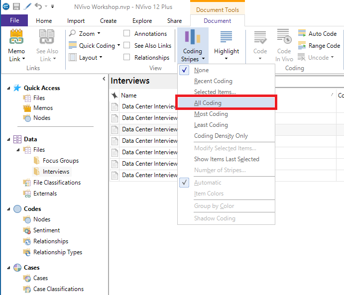
16. From the Document ribbon, select the Coding Stripes drop-down menu and pick All Coding.
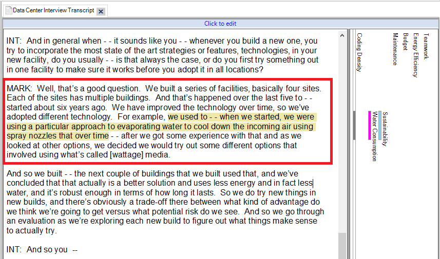
17. You should see coloured stripes along the right to tell you what parts of the document have been coded and how.

18. Next, from the Document ribbon, select the Highlight drop-down menu and pick All Coding.

19. You will see the coded text in yellow highlighting.
Creating Notes
1. Let’s move on to another use of NVivo. You can create different types of notes to capture your thoughts on some text in a file, a file itself, or the project as a whole. Let’s make a note about something that has come up in the text. Open up one of the interview files, highlight some text, right click, and select New Annotation.

2. A small table should pop up at the bottom where you can add your note. Type out a small note, such as “This is important!” When you’re done typing your note, just click on the document again. You will see that annotations are highlighted in blue. Close the file.

3. Let’s say instead that you want to make a note about this whole interview file that you had open. Go to the Interviews folder and right click on an interview file. Select Memo Link and then Link to New Memo.

4. Give your memo a name, such as “Interview Memo” and click OK.

5. You will be given a blank page where you can write a detailed memo about that file. Perhaps, for example, this interview was held in poor conditions, such as a noisy coffee shop, that might have influenced what was talked about. You could note that here.

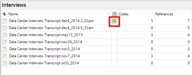
6. Once you close the window, the memo is saved and linked to this file. You should see a small icon next to the interview in the list for the memo link when you have the interview list opened completely (with no other files open to the right of it). To view the memo link, right click on the file again, select Memo Link and then Open Linked Memo.
7. To see annotations you have created all in one place, using the left menu, under Notes, click on Annotations. To see the memo links, under Notes, click on Memos.

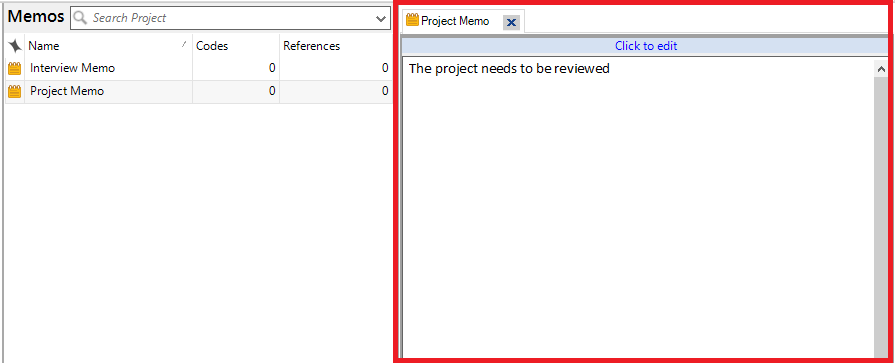
8. Finally, you can also create a note that applies to the entire project, for example, maybe some ideas you have about how the research is going or new themes that are emerging. Right click on Memos and select New Memo.

9. Give it a name, such as “Project Memo” and click on OK.

10. Type some notes, such as “The project needs to be reviewed” and then close it to save. You can always double click on it from the list of memos to re-open it.
Case Classification and Cases
If you have demographics or other important attributes that you want to incorporate into your study, case classifications and cases can help. For example, if you were analyzing interview transcripts, you might want to create a case classification called “Interviewees” with attributes such as their name, age, education, job title, etc. Once your case classification is in place that defines what characteristics you want to capture for your interviewees, you could then create one case for each interviewee with those attributes filled in. So for example, if you interviewed someone named Geeta, you would create a case called Geeta (or some ID number if needed for confidentiality) with information about Geeta. You would then use that Geeta case to code all the files/content that are associated with Geeta (where the Case acts like a node). Later you can then run queries that incorporate that information to answer questions such as, do executives talk more about sustainability? We will talk about how to run queries later in the tutorial.
You can manually create case classifications and cases by using the left menu, under Cases. You can right click on case classification and create a new classification or right click on cases to create a new case. But often times, it is easier and more common to upload a spreadsheet with all the information for the cases. Let’s try that now.
1. For our project, we have a spreadsheet called Interviewees. Open it up in Excel and take a look. It lists our interviewees and their attributes. NVivo would call this a classification sheet. Now close it.

2. Go to the Import ribbon in NVivo and select Classification Sheet.

3. Browse to the Interviewees spreadsheet and click on Next.


4. From the Classification Type drop-down menu, select Case Classification. Keep the rest of the defaults (i.e., everything has a checkmark) and click on Next.

5. Our classification sheet’s first column provides the name of each case (i.e., the interviewee’s first name). So select As names if not already selected. Also keep Create new cases if they do not exist checked so that our cases will be created. Then click on Next.

6. This last step allows us to specify how dates, times and numbers should be imported. We can keep the defaults here. Click on Finish.

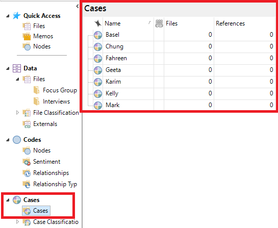
7. Using the left menu, under Cases, click on Cases to see our newly created cases. These cases can now be used in coding the same way nodes are used.
8. We can take advantage of NVivo’s autocoding features to allow us to identify the interviewee’s responses in a file and code them automatically into the appropriate case. Using the left menu, under Data, then Files, go to the Interviews folder and right click on the interview transcript titled “Data Center Interview Transcript oct3_2014”. Select Auto Code…

9. You are presented with a wizard with different autocoding features that I encourage you to explore on your own. For now, let’s select Speaker name. This is going to automatically code text based on speaker name. Then click on Next.

10. Our transcripts are formatted in a consistent manner so we can always pick out who is speaking because the text is labeled as “INT:” for the interviewer’s words, and the person’s name in capital letters followed by a colon for the interviewee’s words. We need to tell NVivo who are all the unique speakers in this document. Under Enter all speakers, type in “INT” and hit Enter. Then type in BASEL and hit the TAB key. You should check the preview below to confirm that NVivo is picking up each unique speaker by highlighting them in different colours. If it looks correct, click on Next.

11. Make sure Add to existing classification is selected and from the drop-down next to it, Interviewees is selected. Then click on Finish. This should code everything that Basel said in the transcript with Basel’s case.

12. Using the left menu, under Cases, click on Cases to see cases again. Double click on the BASEL case. You should see everything that Basel said in his interview. These words are coded to this case. The BASEL case node is now linked to Basel’s interview responses.

Save the Project
1. While NVivo will ask you to save your project every 15 minutes, when you are done working on a project it is important to remember to save manually. From the File Menu, select Save to save the current project.


2. You can also save a project by clicking on the floppy disk icon on the top left, above the file menu.

3. Finally, you can close a project to return to the NVivo main screen. Once your project is saved, go back to the File Menu and select Close.

Part 2 – Queries
In this second part of the tutorial we will be looking at queries. One advantage of putting all your documents and coding in one NVivo project, is that you then have the ability to query the information to gain more insights.
Queries work better for larger projects with a lot of coding already completed, so we’re going to work with the sample project that comes with NVivo for this next section.
Word Frequency and Text Queries
1. First, make sure you have saved and closed any previous projects you had open.
2. From the main screen, select Sample Project. This will open a ready-made project that comes with NVivo. Data in this sample project are drawn from a two-year research study (2008-2009) undertaken by researchers from the Duke University Nicholas School of the Environment at the Duke Marine Laboratory in Beaufort, N.C. The study documented community perceptions of development and land-use change on coastal communities in the Down East area of Carteret County, North Carolina, USA.

3. If a Quick Start Steps window opens up, just close it for now.

4. Let’s see how queries can help us make sense of this project. Go to the Explore tab of the ribbon to see all the queries available to you.

5. PC users have a feature in NVivo called the Query Wizard that helps you decide upon the right query for the right task. It also helps break down the query so that you can understand the different options available. Let’s try that first. Click on Query Wizard.

6. The four options correspond to the first four query types we are going to explore – you can see them named on the right as you select different options. The first two options are great to use near the beginning of a project to get to know your content and help you with coding, the other queries work better once you’ve worked on your project and have done some coding and potentially added cases.
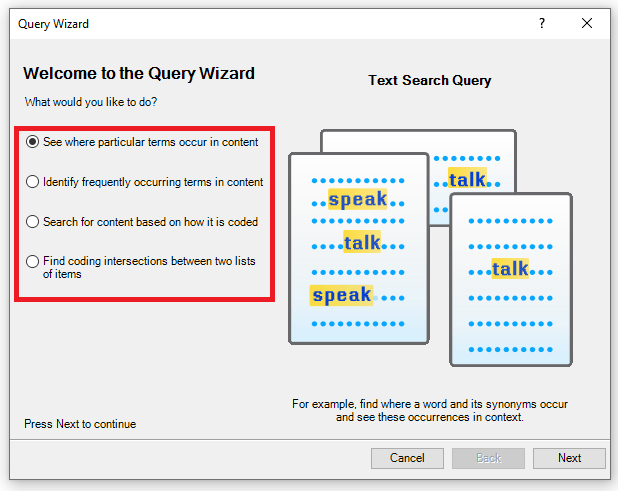
7. Let’s start with the second option – the Word Frequency query, which is described as “Identify frequently occurring terms in content.” If you don’t want to use the query wizard, you could also select Word Frequency from the Explore Ribbon directly. This is a great query to start with to get a sense of the content or topic of your data, by looking at the most common words used in a particular file or your whole project.

8. From the wizard, select the second option and then click on Next.

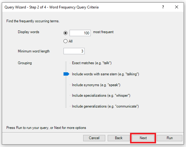
9. From here we can adjust the settings of our word frequency query. Instead of 1000 words, change that to 100. Minimum word length can remain at 3 characters.

10. For grouping, this has some useful settings. If you select the second option, include words with the same stem, it can group a word with all its different word endings together, so they don’t take up distinct spots in our top 100 words. So for example, “run,” “runs,” and “running” would just be grouped together and then tallied once. You could go further and group synonyms, specializations or generalizations, but let’s just select stemming for this example. Drag the slider to the second option to Include words with same stem.

11. Once you’ve made your selections, click on Next.
12. Next, you’re asked where you want to search. This is a common setting for most queries. The default option is to search everywhere in the project. You could however, select particular files or folders that you want to search by choosing the second or third options. For example, if we only want to search Interviews, and we’ve been very organized and put all of our interview transcripts into a folder called Interviews, we could select the third option. However, our interview folder has a combination of text, plus audio and video files. If we want to only select the text transcripts, we’d select the second option. Let’s try that. Choose Selected Items and click on the Select… button.

13. Then expand Files in the folder tree to see our interview folder and select it to view its contents. Put a checkmark next to the Interviews folder to select everything in that folder to start, but then unselect 2 videos and 1 audio file (they have different icons). So only the text transcripts should be selected for our search. Then click on OK.

14. Then click on Next.

15. Next, you’re asked if you just want to run this query once, or if you want to save it and add it to your project in the Search section on the left because you could see yourself running this query often. In this case, let’s just run it once, but later we will save a query that we want to revisit. Leave the defaults and click on Run.

16. Now we should see the results of our query. You should see a list of the top most common words in our interview transcripts, sorted with most common at the top. It tells you how many times the word (or group of similar words in our case) occurred and the last column shows you what words were grouped together.
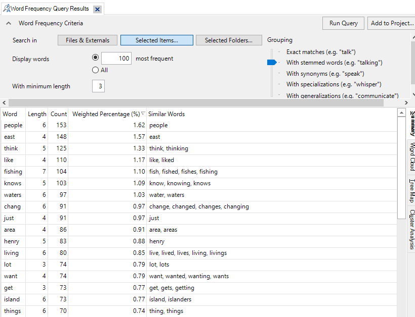
17. Word frequency lists normally ignore stop words, which are really common words that wouldn’t be useful to analysis. For English, these are words like “a,” “the,” “and,” etc. When you’re looking at this list of results, if you see a word that doesn’t really have much meaning in this context, such as “things,” you could add it to the stop words list and re-run the query so it’ll ignore it. To do this, right click on “things” and select Add To Stop Words List. As we had stemming turned on, it presents you with all the words you’ll be adding to the Stop Words list to check. You can remove individual words from this list if you want. When you’re ready, click on OK. Then click on Run Query at the top right to re-run the query. You should see that “things” is now missing from the list.

18. To see the Stop Words list, and even reset it, go to File, and select Project Properties on the right, under Project Information.

19. Here you can select the Text Content Language. The default is English (US), but you can see other options. This doesn’t affect the interface, but is important for certain queries, such as word frequency queries and affects the stop words list. So for example, you could have an English interface for NVivo, but be analyzing interview transcripts that are in French, by selecting French here. Click on the Stop Words button to see the list of stop words in use. From here, you could select reset to reset the list to the default, if you wish. Let’s just click cancel twice for now and go back to the results of our query.


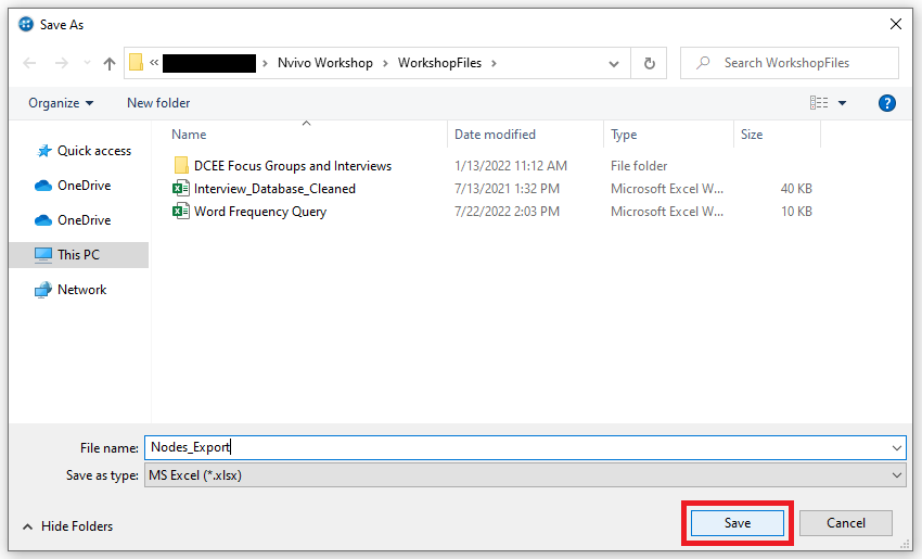
20. You can also export these results into a spreadsheet. Right click on the table and select Export List.

21. Browse to the workshop folder, give the file a name or keep the default and click on Save.

22. If we go back to the query results, on the right hand side, you will see 4 tabs. We are in the summary tab. Click on Word Cloud.

23. This shows the more frequent words, where the larger the word is, the more frequently it occurs, which is a common way to display this type of result. (Might take a few seconds to load).
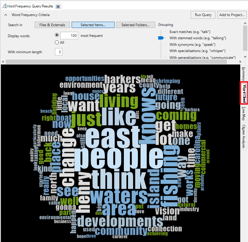
24. On the ribbon at the top, you will see a new context-specific section called Query Tools that gives you different themes you can choose to customize your word cloud.

25. You can also right click on the word cloud and export it as an image or PDF to use later in a report.

26. Also, if you double click on any word in the word cloud, you’re given a list displaying each instance of the word in context.

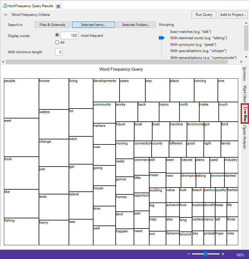
27. Go back to the word frequency query results window. Click on the third tab, Tree Map. A Tree Map is an alternative visualization for word frequencies. The size of the rectangle is proportional to the frequency, and the most frequent word will always be found in the top left corner, and the least frequent will be in the bottom right corner. Tree maps are more commonly used to show parts to whole with hierarchies (so a more complex rectangular pie chart), so then are not ideal for visualizing word frequency.
28. Click on the final tab, Cluster Analysis. This is a visualization where words that co-occur are clustered together in a hierarchical tree diagram called a dendrogram. You can zoom in using the slider on the bottom right. You can browse to see if there are some surprising groupings.

Note: NVivo’s visualization options are limited, and you can often get better visualizations by exporting your query results and importing them into other tools more suited for data visualization. If you’re interested in learning more tools and techniques for this, check out our data visualization guide!
29. Once you’re done looking at the results of a query, you can just click on the x to close the query results window.

30. Next, let’s look at the Text Search query, which is described as “See where particular terms occur in the content” if you are using the query wizard. But this time, let’s select it from the Explore Ribbon directly. Click on Text Search.

31. You can use it to find a word or phrase. You can search for phrases by putting them in quotation marks. Let’s try looking for mentions of "family". Type “family” in the search box and choose With stemmed words, so that it will also search for “families” similar to what we did in the Word Frequency query.
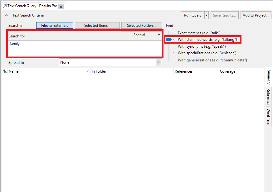
32. Next, we select where it should search. As before, the default is all the documents in the project. Let’s keep the default this time and just run the query. Click on Run Query.

33. You will be presented with a list of project files that contain that reference. You can double click on a file to see the references. Try that with the item called “Susan,” which you can see has 6 references.
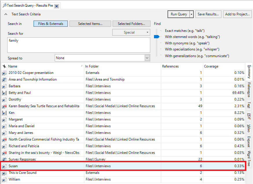
34. This opens up Susan’s interview transcript. You can use this to help find references that you might want to code.

35. If you go back to the query results, you will see on the right, the Reference tab. You can click on the Reference tab to see all of the references together in one page.

36. Other tabs on the right, such as text, PDF, video and dataset, only show you references in that type of content, to narrow down your search.

37. Click on the final tab, Word Tree, which shows you what words often come before and after the term or phrase you searched for. This is useful to understand how that word or phrase is being used.
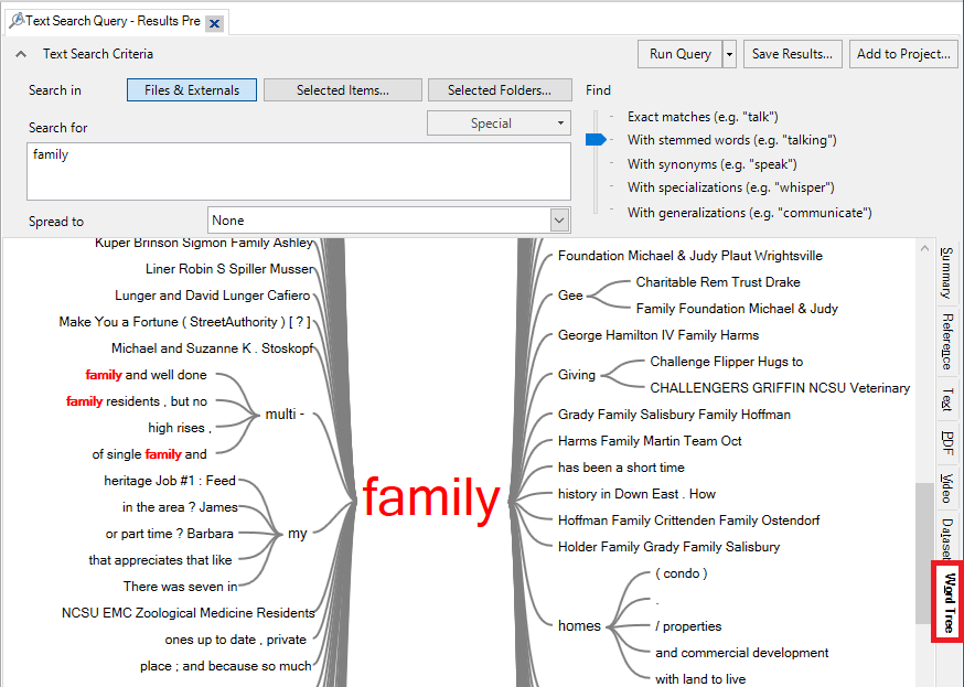
38. You can save the results of this query. Click on Save Results… at the top right.

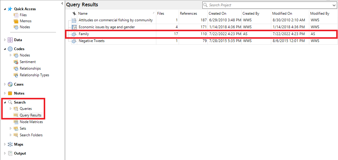
39. You will notice at the top of the pop-up window that this is not just going to save the results, but also create a new node, and code the results based on that node, with the node called what we name the query results. This node only lives in the Query Results folder, but you can copy it and add it to your nodes list if you want to use it for more coding. Also note that these results are just a snapshot and don’t dynamically change if the project items change. Let’s save our results. Call it “Family” and click on OK.

40. Close the Query results tab. Then using the left menu, under Search, go to the Query Results folder. You will see the Family query results saved, and you can double click on it to view the results again. Unfortunately, the Word Tree won’t be saved here.
Test Your Understanding 1
Using either the Query Wizard or the Explore ribbon options run a Word Frequency query for the project to find the top 50 words, grouping synonyms. Only search News Articles. What was the most common word?
Next run a Text query for the project to find the phrase “climate change” in all project items. How many project items were in the results?
Click here for the answers.
Coding Queries
1. Okay, now let’s move on. Close any query results tabs that you have open.
2. The next few queries I am going to show you are better to use when you have done some coding, as they can help you gain insight from all your work coding your content. For example, you could use these to find potential connections between themes, or connections between a theme and a certain demographic.
3. Let’s start with Coding queries. You can use these to find all content coded at selected nodes, a combination of nodes, or a combination of nodes and attributes. It is called Coding in the Explore Ribbon or described as “Search for content based on how it is coded” in the Query Wizard. So for example, let’s say you want to see if there is content coded as both “memorable quote” and “real estate development,” and you only want to see references that are from residents of Marshallberg – you can do this with a Coding query. Let’s access it through the Explore Ribbon, as we can create a more complex query that way; click on Coding.

4. We can keep the defaults for now, which only finds references that are coded with all the codes listed. So we just need to click on the ‘…’ button next to the All Selected Codes or Cases dropdown menu to select the two codes we want.
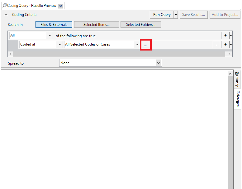
5. Select “Memorable quote” and “Real estate development.” Then click OK.

6. Now let’s click on Run Query to see the results.

7. You are shown all the results, but you can also click on the Summary tab to see how many results you got. We can see there are a few results in interviews and survey responses.

8. We can narrow this down further, to just quotes from residents of Marshallberg. To do that, click on the plus sign at the top right to add another parameter to our search.

9. For this new row, we use the All Selected Codes or Cases drop-down menu to select Any case where.

10. Next click on the … button.
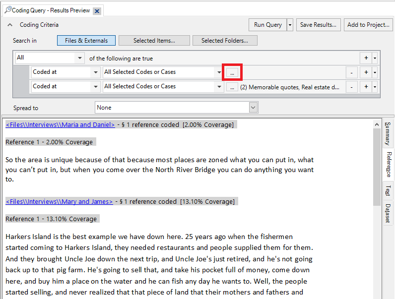
11. Then expand Person, select Township, and click OK.
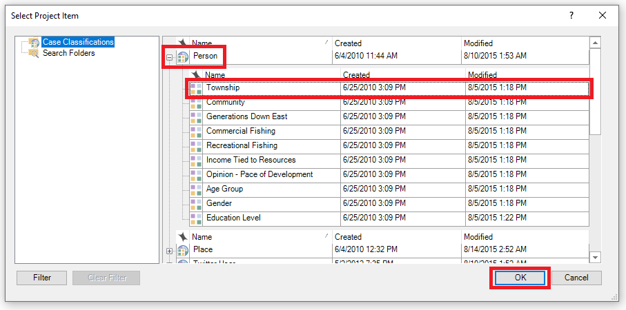
12. From the far right drop-down, select “Marshallberg.” (You might have to scroll to the right to see this.) So the query says “All” at the top left, meaning all of these conditions must be true. Then one line says that the content must be coded with both nodes, Memorable quotes and Real estate, and then the other line says AND the person who said this must be from Marshallberg.

13. Click on Run Query again. This time you can see we get just one large memorable quote on real estate from Mary and James, who are from Marshallberg.

14. We might not want to save the results, but we might want to save this query to re-run again in the future as we continue to code. To do that, click on Add to Project at the top right.

15. Give it the name “Marshallberg Quotes on Real Estate” and click on OK. Then close the query results tab.

16. This query is now saved in the Search section on the left, under Queries. You can double click on it at any time to re-run the query.

Test Your Understanding 2
Using the Explore ribbon option run a Coding query for the project to find interview content coded as “Infrastructure,” “Policy, management,” OR “Real estate development” where the interviewees are from Harkers Island. How many references did you find?
(Hint: You will have to change an option to say Any instead of All to satisfy the “or” condition, different than in the demonstration.)
Click here for the answers.
Matrix Coding and Crosstab Queries
1. Next up are Matrix Coding queries. These allow you to see coding intersections between two lists of items. It is called Matrix Coding in the Explore Ribbon or described as “Find coding intersections between two lists of items” in the Query Wizard. So for example, let’s say you want to see which interviewees (based on cases) had the most positive and negative attitudes (based on coding) - you can do this with a Matrix Coding query. Let’s access it through the Explore Ribbon; click on Matrix Coding.

2. This query is formed using drag and drop. First, using the left menu, under Cases, go to People, and then expand Interview Participants.

3. Highlight all of the interviewees by clicking on the first one, holding down the Shift key, and then clicking on the last one. Then drag and drop them on the left side of the matrix query under Rows.

4. Then, using the left menu, under Codes, click on Nodes, and then go to Attitude and expand it.

5. Highlight all the attitude child nodes and then drag and drop them on the right side of the matrix query under Columns.

6. Click on Run Query to see the results. You will see a grid or matrix with the number of references where those nodes and cases intersect.

7. To see the results more clearly and point out interesting patterns, use the shading options available from the top left of the Matrix Tools ribbon. Select the purple option.

8. We can see that the darker the purple, the more two items intersect. In this case, we can see for example that Barbara had strong positive and negative references, Thomas’s interview was more negative than positive, and William’s was only positive.

9. Click on the Chart tab on the right.

10. You will see the results displayed in a chart. The default is a 3D bar graph.

11. You can select other chart types from the Matrix Tools ribbon above to change it. Again, NVivo’s visualization options are limited, and these graphs are often not the best way to display your data. In this scenario the shaded matrix view offers a clear visualization of the data.

12. Click on the Node Matrix tab on the right. Then right click on the table, and go to Cell Contents, you will see that the default number shown is coding references, but there are a lot of other options to consider to explore the data in different ways. For example, change it to Words Coded, you can see that Charles had a lot of negative things to say. Once you have finished examining the results, close the query results tab.

13. Let’s move on to the last query we will look at today, Crosstab queries. Crosstab queries are similar to Matrix Coding queries, but you can expand out all the categories for an attribute along the columns automatically. For example, to determine which themes were discussed most by Township of respondent. Let’s access it through the Explore Ribbon; click on Crosstab.

14. This query is partially formed using drag and drop. First, using the left menu, under Codes, go to Nodes. Highlight all the top-level nodes (make sure none of the Node categories are expanded) and then drag and drop them on the left side of the Crosstab query tab under Codes.

15. The default option for the Crosstab codes against is attributes. For Classification, select Person, and for Attribute 1, select Township, from the drop-down menus. This Crosstab query will create a matrix where the codes are along the rows, and for the columns, it will take all the values of one attribute (in this case, Township) and use those for the column headers. Then it will tally where they intersect.

16. Click on Run Query to see the results. You will see a matrix with the number of references where those nodes and attributes intersect.

17. Like with the Matrix Coding, use the shading options available from the top left of the Crosstab Tools ribbon to see the patterns more clearly. If we select the leftmost green option, we can see that the darker the green, the more two items intersect.


18. Again, we can right click on the table, and go to Cell Contents to change what is displayed. In this case, try selecting Coding Presence. Often times you might not have a big enough data set to gain meaning from the numerical values for coding references, for example, but you can at least see where there is an intersection at all or not. For example, we see that the theme of a “Sense of Community” has only been used on data for a few townships. Normally people don’t report these numbers, but use them to gain insight into their project.


19. You’ll see that NVivo also offers three other query types: Coding Comparison Queries, which are used when working on a team to see how much agreement there is between team members on coding, and Compound and Group Queries that are used to create more complicated queries combining elements from the other query types we have discussed. While these will not be covered in this tutorial, you are encouraged to play around with these queries on your own time to learn more.
Test Your Understanding 3
Using the Explore ribbon options run a Matrix Coding query on social media content only, where the columns are the attitude child nodes (positive, negative, etc.) and the rows are the remaining top-level nodes (Balance, Economy, etc). What two nodes have the most negative references?
Next run a Crosstab query, where the rows are the top-level nodes (Balance, Economy, etc) and the Person attribute is Education Level. What node was coded the most by coding references for people whose highest level of education completed is undergraduate college?
Click here for the answers.
Export Data
1. We’re already discussed how you can export the results of your queries, but you can also export your nodes as a list or its references. To export your full list of nodes, first open up your Nodes list and select at least one node. Go to the Share ribbon at the top and select Export List. This will save all of your nodes in a spreadsheet. It will include the number of files coded with that node, and the number of references.

2. Browse to your workshop folder, name your file or keep the default and click on Save.
3. You can also export your codebook, which lists your nodes and their descriptions to understand when a node is normally used. Again, go to the Share ribbon at the top and select Export Codebook.

4. Select Include number of files and references. This creates a Word document with this information. Keep the defaults and click on OK.

5. Finally, you can also export all the references for a particular set of nodes. To do this, first select your subset of nodes. For example, select Balance and Community Change.
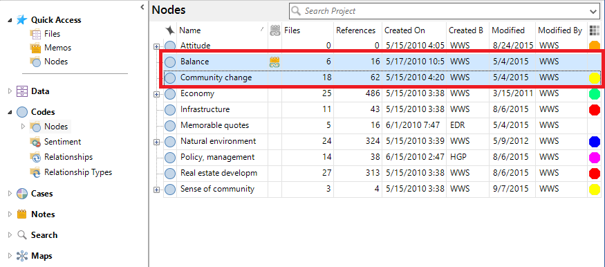
6. Then go to the Share ribbon at the top and select Export.

7. From this window, you have three options. You can select Entire Content, which creates a local website where you can navigate through all the references, but I don’t find this to be a useful option. Instead I would recommend either Reference View or Summary View. Reference View creates a list of each reference, similar to what you would see if you double clicked on the node. You can save this list as a Word document, text file or PDF. Summary View provides a table that shows you how many times that node was coded by project item. You can save this list as an Excel file, Word document, text file or PDF. Try saving both the reference view and summary view formats. Open up all the files you have exported to see their contents.

And that's it!
Resources to Learn More
Visit our Getting Started page for more information, tutorials, and workshops on NVivo 12!
Qualitative Research Methods
Qualitative Data Analysis and Coding
NVivo
Related Information
Test your Understanding Answers
- The most common word is variations of the word "take". It appears through the news articles 28 times. [Note: The word "oyster" comes up first in the list, but only has 26 references. If you click on the Count column, it'll sort properly to show you the top word. This is unusual behaviour, though. I think this is a bug in NVivo.]
- A Text query for the project to find the phrase “climate change” in all project items has 5 project items.
- Back to the next section.
Test Your Understanding 2:
- There are 15 references total. Robert’s interview has 6, Susan’s has 4, and Thomas’ has 5.
- Back to the next section.
Test Your Understanding 3:
- The Natural Environment Node has the most negative references with 33, followed by Economy with 27.
- The nodes coded the most by coding references for people whose highest level of education completed is undergraduate college is Real Estate Development, with 51 references.
- Back to the next section.