This guide has been created using Stata IC version 16.1. The main dataset used is the flights dataset. It contains the US domestic flights in January 2020 [1]. The other two datasets used are fabricated datasets created for the purpose of this guide.
The link to the recording of this workshop can be found here. Additional resources are listed below. If you need assistance, fill out the support request form.
TABLE OF CONTENTS
Getting Started
Importing Data
Exploring Data
Graphs
New Variables
Managing Data
Reshaping Data
Stata Packages
Resources
Getting Started
There are three ways to run tasks in Stata. You can use point-and-click to execute tasks using the dialogs from the Data, Graphics and Statistics menus.
You can type Stata code in the command window and submit the code by hitting the ENTER/return key.
Or you can type Stata code in the do-file editor. To open a do-file editor, go to the File menu, then go to New and select Do-file. Once you type your code in the do-file, you can run it by highlighting the line of code and clicking on the execute icon (the play button) in the top-right corner of the do-file window.
The results will always appear in the results window. Stata is case-sensitive.
Some useful commands to get started:
search enter_topic_here returns the list of commands associated with a topic
help enter_command_here returns the help file for a specific command
clear removes the dataset that is currently loaded in memory so that you can import a new dataset
Importing Data
Working directory
The working directory is the home directory that Stata works from by default. Pwd gives the current working directory. Use cd to change the working directory to the location of your datasets. You are advised to save all the datasets from this tutorial in the same folder and to make this folder the working directory using the cd command.
Dir and ls both show the content of the current directory.
pwd
cd "[enter path here]"
dir
ls
Importing Data
DATA: flights.dta
Download the flights dataset by clicking on the link above or using the url uoft.me/flightsstata.
The use command can be used to import a Stata dataset. Every time you import a dataset, it is good practice to add the clear option to clear any dataset that is loaded in memory. Options are added after the comma.
use flights, clear
Once you import the dataset, the variables are listed in the variables window. You can check the number of rows and the number of observations in the properties window.
Exploring Data
Describe enumerates the list variables, their data type and their labels. Codebook gives a frequency table for character variables, basic statistics (mean, std dev etc) for numeric variables and the number of missing observations for both types of variables.
describe
codebook
List can be used to print data values in the results window. It allows users to specify the variables and observations to print.
list originstate in 1
list originstate deptime depdelay in 1000/1005
Tab is an abbreviation for tabulate. The m option is used to display the number of missing values for the specified variables. The cell, row and col options display the cell, row and column percentages.
tab depdelay, m
tab depdelay arrdelay, m
tab depdelay arrdelay, m cell row col
Sum is an abbreviation for summarize. It gives summary statistics of numeric variables. We can add conditions to a line of code using the if qualifier. For example, we can get the summary statistics of flight distance for flights that took place on Mondays only using the dayofweek variable and setting it equal to 1 which represents Monday. Two equal signs are used for the equal to condition.
sum distance
sum distance if dayofweek==1
Bysort can be used to run a line of code for every category of a second variable. For example, we can get the summary statistics of flight distance for each day of the week.
bysort dayofweek: sum distance
Graphs
The hist, scatter and graph bar commands can be used to make a histogram, a scatterplot and a bar chart respectively. There are many options that can be added to modify all graphs. These options come after the comma. The list of options possible can be found in the help file of each command. Some options can be applied for all or most graphing commands. Title() can be used to add a main title. Xtitle() is used to specify the label of the x-axis. Ytitle() is used to specify the label of the y-axis.
The normal option adds a normal curve on the histogram. Bin() allows the user to specify the number of bins. Color() and lcolor() are used to specify the color of the bin and the border around the bin.
hist deptime
hist deptime, normal bin(30) color(ltblue) lcolor(white) xtitle(Departure Time)

The msymbol(), msize() and mcolor() options can be used to specify the shape, size and color of each point on the scatterplot. The xlabel() is specify the ticks on the x-axis. The plotregion() is used to specify the margin between the plot region and the axes.
scatter deptime dayofweek
scatter deptime dayofweek, msymbol(+) msize(huge) mcolor(maroon) xlabel(1(1)7) plotregion(margin(10 10 2 2))

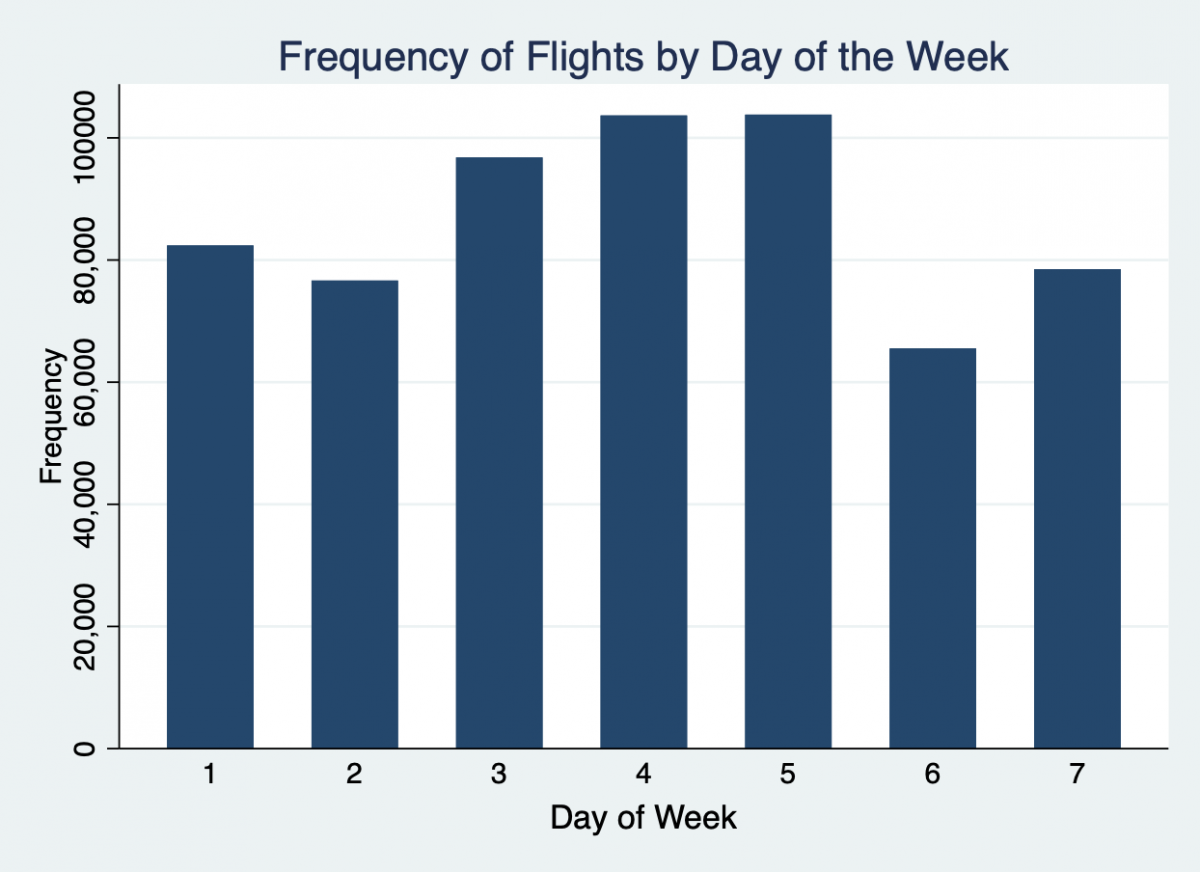
The bar chart is usually used to plot summary statistics on the y-axis such as the number of observations for each category of another variable. The count statistic is specified in parenthesis to make a bar chart of the count of observations. The variable on the x-axis is specified in the over() option. B1title() is used to label the x-axis of bar charts instead of xtitle().
graph bar (count), over(dayofweek)
graph bar (count), over(dayofweek) title(Frequency of Flights by Day of the Week) ytitle(Frequency) b1title(Day of Week)

You can continue a line of code over multiple lines by adding three forward slashes at the end of the lines that continue.
New Variables
To generate a new variable that is a function of other variables, use the generate command. You will find a few examples of how to create different types of variables below. In the first example, the variable distancemiles (distance in units of miles) is created by converting distance in kilometers to miles.
* Example 1
gen distancemiles = distance * 0.621
sum distance distancemiles
* Example 2
gen instate = .
replace instate = 1 if originstate==deststate
replace instate = 0 if originstate!=deststate
tab instate, m
Labels can be created for the entire dataset, for a variable and for the levels of a categorical variable. To label the levels of the variable instate, first the label instatelabel is created using the label define command. Then it is assigned to the variable instate using the label values command.
label define instatelabel 1 "Within State" 0 "Between State"
label values instate instatelabel
tab instate, m
* Example 3
gen delay = ""
replace delay = "not delayed" if depdelay==0 & arrdelay==0
replace delay = "delayed at departure only" if depdelay==1 & arrdelay==0
replace delay = "delayed at arrival only" if depdelay==0 & arrdelay==1
replace delay = "delayed at both" if depdelay==1 & arrdelay==1
tab delay, m
The command egen is used to generate new variables using built-in functions. For example, the mean() function generates mean. Example 4 creates a new variable called meandistance that is the mean of distance. Example 5 creates a new variable meandistancebycarrier which is the mean distance for each carrier or airline.
* Example 4
egen meandistance = mean(distance)
tab meandistance
* Example 5
egen meandistancebycarrier = mean(distance), by(carrier)
tab meandistancebycarrier
The original flights dataset now has 5 new variables. This can be checked in the variables window. The save command can be used to save this flights dataset. It is good practice to use the replace option.
save flights.dta, replace
Managing Data
Subsetting Data
Keep can be used to extract a part of the dataset. You can extract specific variables or observations based on criteria.
* Subsetting Data : Variables
use flights, clear
keep originstate origin deptime depdelay deststate
save departure, replace
* Subsetting Data : Observations
use flights, clear
keep if deststate=="Hawaii" & dayofmonth==1
save hawaii, replace
Merging Data
DATA: airlinecodes.xlsx
Download the airlines dataset by clicking on the link above or using the url uoft.me/airlinesexcel.
To merge two datasets, sort each one by the merging variable first then use the merge command to combine them. Whenever you merge two data files, a variable called _merge is created in the merged dataset. This variable helps you identify the observations that were successfully merged.
use flights, clear
sort carrier
save flights, replace
import excel using "airlinecodes.xlsx", clear firstrow
sort carrier
merge carrier using flights
save flightsmerged, replace
tab _merge
tab airline diverted, row
Exporting Data
In this section, we create two new variables departureflights and arrivalflights that represent the total number of departing and arriving flights for each airport using _N. This total will be repeated in every row for a particular airport. To obtain a simple table of these totals by airport, we use the collapse command to shrink the dataset to contain only the first value of departureflights and arrivalflights variables for each airport. Then we export this dataset as an excel file using the export excel command.
The commands preserve and restore are used to temporarily modify a dataset and export it before returning back to the way the dataset was before the preserve command. In our example, after the airport dataset is created and exported, it returns us back to the flights dataset. For this code to work, you will need to run the lines from preserve to restore together.
use flights, clear
bysort origin : gen departureflights = _N
bysort dest : gen arrivalflights = _N
gen airport = origin
preserve
collapse (first) departureflights (first) arrivalflights, by(airport)
export excel "Airports.xlsx", replace firstrow(var)
restore
Reshaping Data
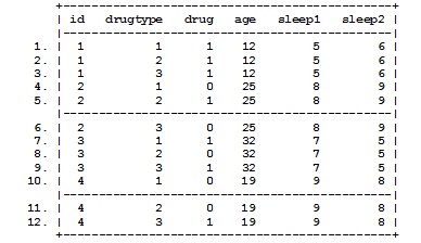
To reshape a data set between wide and long format, use the reshape long or reshape wide commands. For a data set in wide format, the variables that denote the repetition should be named with the variable name followed by a number (i.e. variablename#). For example, in our data set we have drug1, drug2 and drug3. The numbers do not need to be consecutive.
clear
use https://maps.library.utoronto.ca/workshops/Stata1/statawide, clear
list

describe
list
reshape long drug, i(id) j(drugtype)
list

table drugtype, contents(n drug mean drug sd drug)

reshape wide
list
Stata Packages
The ssc install command can be used to install packages from the SSC archive.
ado dir
ssc install outreg2
ado dir
Resources
[1] The flights dataset is modified from the original version on the Kraggle website.
[2] Additional resources to learn Stata.
[3] The tutorial code and the workshop Powerpoint presentation can be downloaded from here.
author Nadia Muhe, Map and Data Library, University of Toronto.